Week 4 - CHT Analysis on Exhaust port

AIM:

To run simulation to analyse CHT on exhaust port.

OBJECTIVE:

1. Brief description about why and where CHT analysis is used.
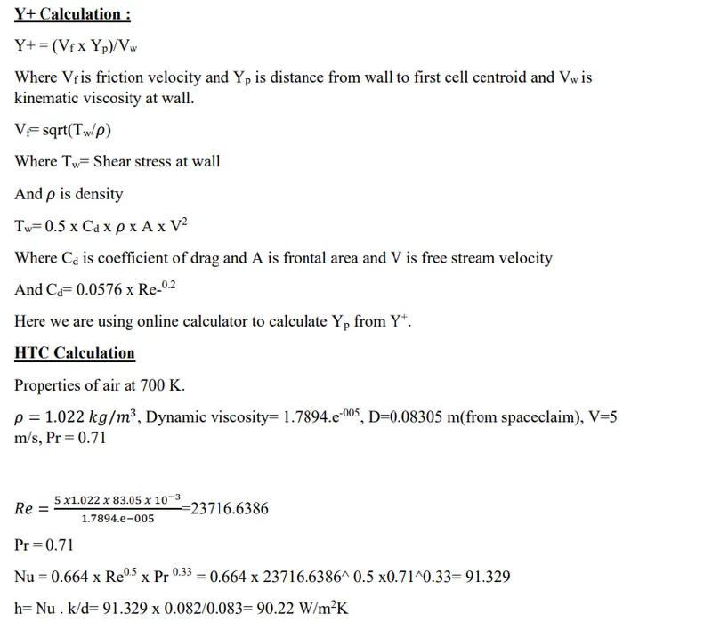
2. Maintain the y+ value according to the turbulence model and justify the results.

1. Calculate the wall/surface heat transfer coefficient on the internal solid surface & show the velocity & temperature contours in appropriate areas.

4. Verify if the HTC predictions from the simulations are right? On what factors does the accuracy of the prediction depend on?

INTRODUCTION:

Conjugate Heat Transfer (CHT)

The term conjugate heat transfer is used to describe processes which involve variations of temperature within solids and fluids, due to thermal interaction between the solids and fluids. A typical example is the heating or cooling of a solid object by the flow of air in which it is immersed.

Applications

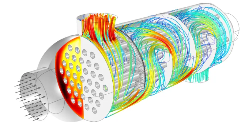
1. Flow and heat transfer analysis of different fluids in heat exchangers can be easily predicted and visualised using simulation softwares.
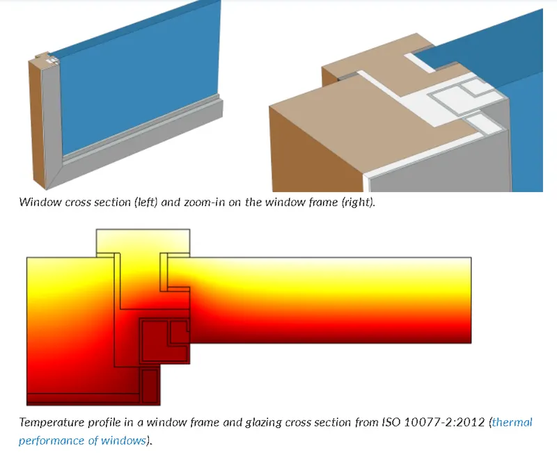
2. Window designing and HVAC conditions where adverse temperature gradients are required are simulated using simulation softwares.
3. Electronic chip cooling and heat sink generation is another major field where CHT analysis is carried out.

THEORY: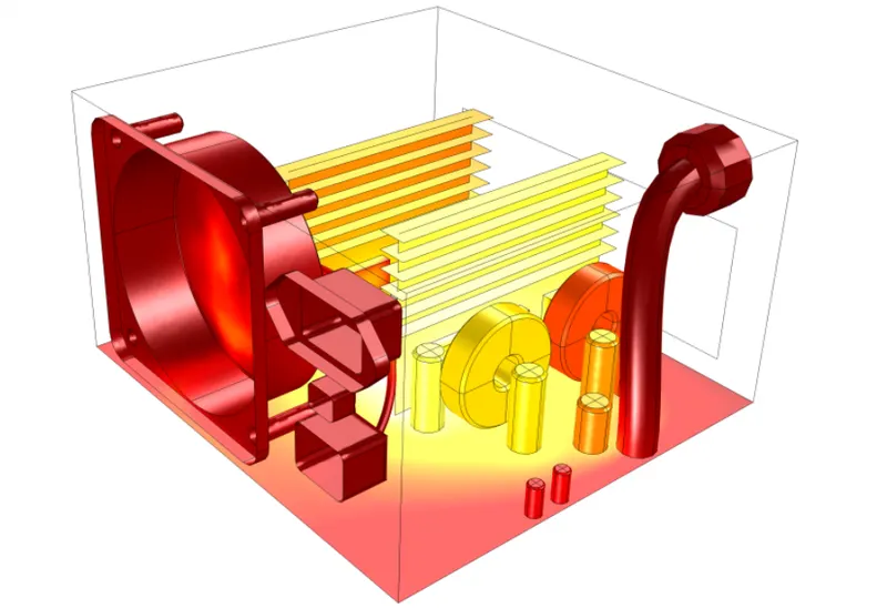

Reynold’s number:

Reynolds number is the ratio of inertia force to viscous force.

PROCEDURE:

SOLVING AND MODELLING APPROACH:

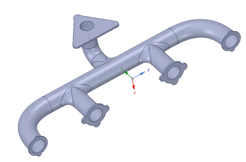
1. Geometry is fed to spaceclaim
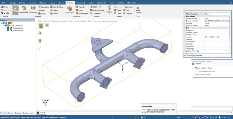
2. Extract volume using edge selection and create new component from solid and fluid volume and make final geometry and delete free geometry.
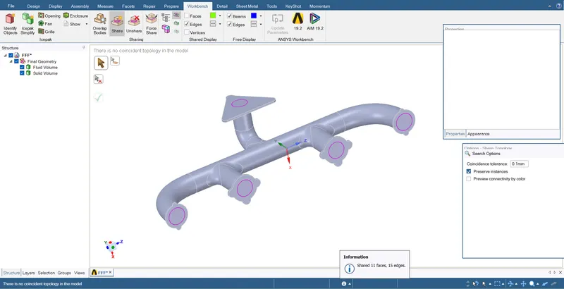
3. Now select share topology and to share the physics between the fluid and solid volume and conformal mesh can be achieved, pink circle are seen after completing the process.

PREPROCESSING AND SOLVER SETTING:

MESH SETTING:

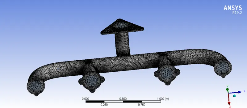
1. Open the mesh and select named selections and name all parts.
2. Run baseline mesh.
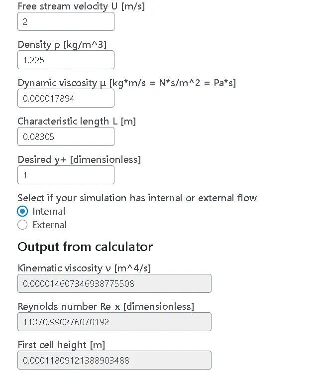
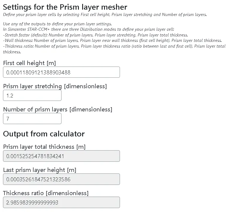
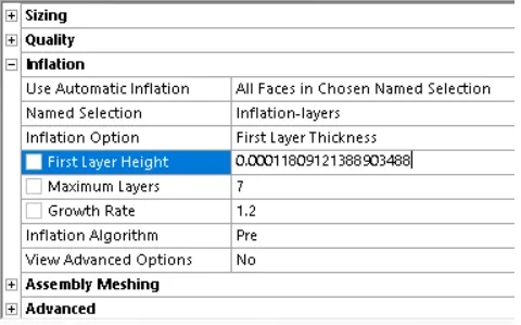
3. Calculate y+ and give inflation layers accordingly and set default element size to 0.01 m to capture more details.

SOLVER SETTING (Steady State):

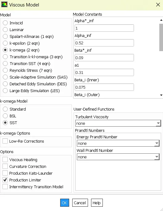
1. Model:Pressure based – Steady state flow, Viscous -SST K-Omega selected.
2. Materials= Air, Aluminium with default settings
3. Boundary Conditions:
   1. Inlet- velocity with magnitude 5m/s and temperature to 700K.
   2. Outlet- Pressure based- Gauge pressure 0
   3. Cylinder wall- Heat transfer coefficient= 20 W/m²K
   4. All other walls with adiabatic condition.

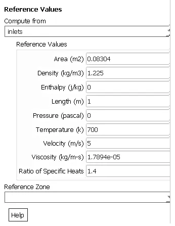
4. Reference values -
5. Method: SIMPLE Algorithm with default wall conditions..
6. Selected Hybrid Initialization and Initialized for 10 iterations.
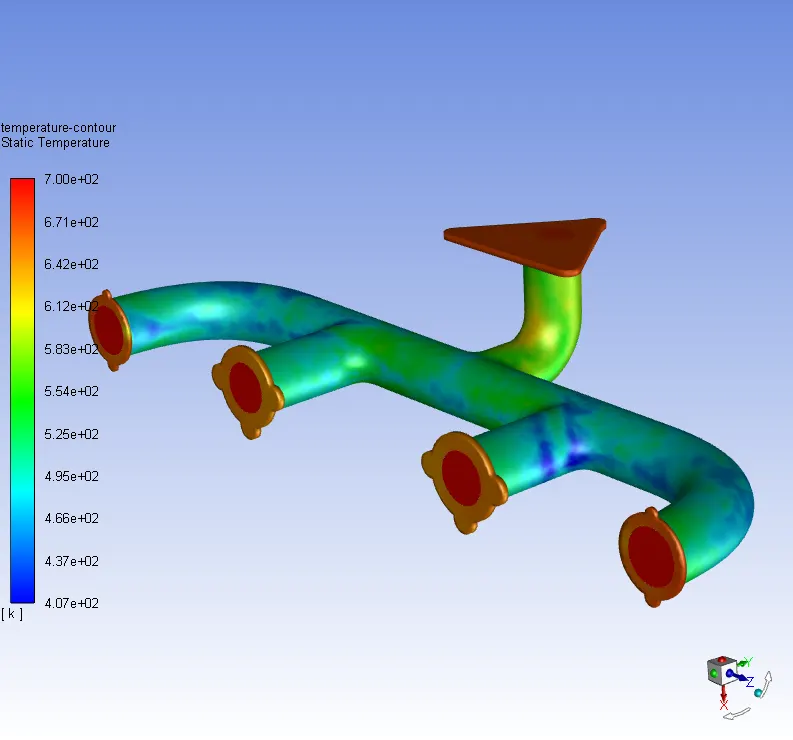
7. Defined new temperature contour plots for temeperature plot.
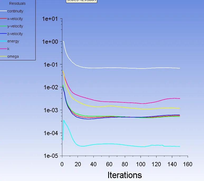
8. Set 150 iterations and run calculations.

POST PROCESSING

1. Open CFD post.
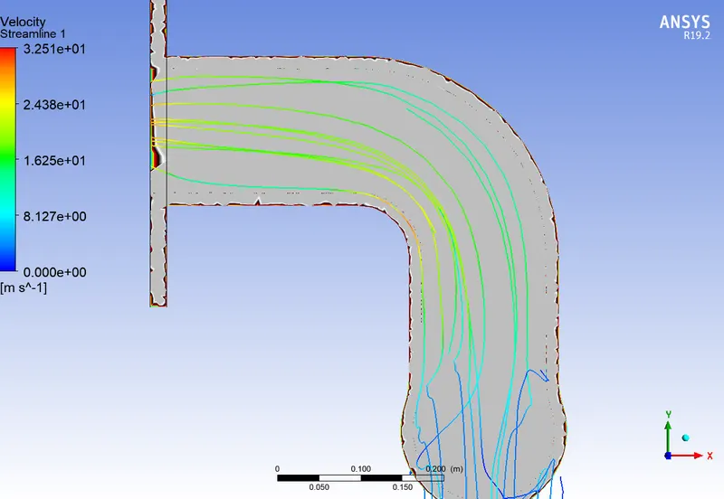
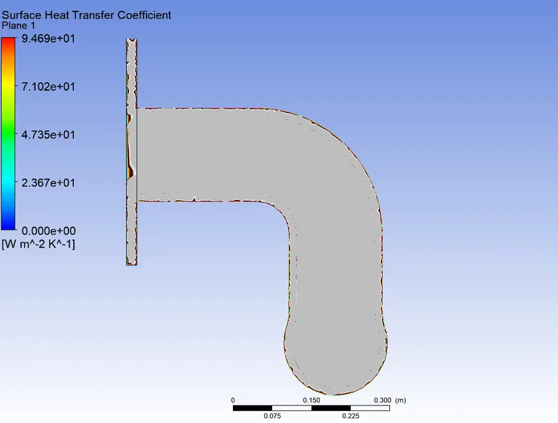
2. Create plane and view wall heat transfer coefficient and velocity stream lines.

RESULT:

STEADY STATE

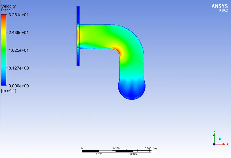
Steady state residuals, temperature, velocity planes, velocity streamline and wall heat transfer are made.

CONCLUSION:

It is noted that from the graph CHT obtained was 94.69 W/m² K and from numerical calculation value obtained are 90.22 W/m² K

As per our results, heat transfer coefficient is high for higher value of velocity and hence from above discussion we think that our results are correct. Thus HTC predictions from the simulations are right.

Thus Accuracy of prediction depends on mesh size, prefect inflation layer and boundary conditions and proper selection of boundary conditions.

Mesh Refinement	Wall heat transfer	HTC from numericals	Error %
Refined Mesh (SST K-Omega)	94.69 W/m2 K	90.22 W/m2 K	4.95%

REFERENCES:

1. https://www.comsol.com/blogs/conjugate-heat-transfer/
2. https://www.quora.com/What-is-conjugate-heat-transfer