Week 4 - CHT Analysis on Exhaust port

AIM :

To perform the CFD simulation on the exhaust port and the analysis is CHT analysis.

ODJECTIVE :

* To perform the CFD simulation on the exhaust port and the analysis is CHT analysis.

* To explain about the CHT analysis which is used in these.

* To Calculate the wall/surface heat transfer coefficient on the internal solid surface & show the velocity & temperature contours in appropriate areas.

* To verify the predicted simulation value using the analytical method.

THEOREY :

CONJUGATE HEAT TRANSFER :

Conjugate heat transfer is a type of heat transfer analysis between solids and fluid(s). This type of heat transfer includes both convection (between fluids) and conductive (between solids) heat transfer, as well as both forced and natural convection.

Typical applications of this analysis type exist as, but are not limited to, the simulation of heat exchangers, cooling of electronic equipment, and general-purpose cooling and heating systems.

Some common examples where conjugate heat transfer analysis if performed are :

* Heat exchanger analysis :

Consider a shell and tube heat exchanger where heat from the fluid at high temperature is transferred to the fluid at low temperature. In the process, heat gets transferred from hot fluid to the walls of the tubes and to the cold fluid. The processes happeining here are convective heat transfer from hot liquid to the walls, conductive heat transfer from face of the wall in contact with the hot fluid and convective heat transfer from other face of the wall to the cold fluid.

* Heat sink :

A heat sink is a passive heat exchanger that transfers the heat generated by an electronic or a mechanical device to a fluid medium, often air or a liquid coolant, where it is dissipated away from the device, thereby allowing regulation of the device's temperature. In computers, heat sinks are used to cool CPUs, GPUs and some chipsets and RAM modules. Heat sinks are used with high-power semiconductor devices such as power transistors and optoelectronics such as lasers and light emitting diodes (LEDs), where the heat dissipation ability of the component itself is insufficient to moderate its temperature.

The three main modes of heat transfer:

* Conduction is heat transfer that occurs when a temperature difference exists across a stationary medium.

* Convection is the heat transfer between a surface and a moving fluid when there is a temperature difference between the two.

* Radiation(thermal radiation) is the emission of energy in the form of electromagnetic waves. In the absence of an intervening medium ,there is net heat transfer by radiation between two surfaces at different temperatures.

Concept of Y Plus :

The Y plus is a dimensionless quantity. It is a distance measured normal to the wall in terms of viscous lengths.

The exact need for the Y plus is to distinguish different regions near the wall like Viscous sublayer, buffer layer, ovelap layer and turbulent layer.

Steps to calculate the first cell height :

1. Determine the value of the Reynolds number.

Re = (rho*v*L)/(mu). Here V is the flow velocity, rhois the fluid density, L is the characteristic length and muis the absolute viscosity.

2. As per the definition of Y+

Y+ = (rho*U_t*Dely_1)/mu

Rearranging for Delta y_1 we get

Delta y_1= (y+* mu)/(rho*U_t) -----(a)

where, U_t is the frictional velocity which can be calculated by the formula:

U_t = sqrt((tau_w)/(rho))

tau_w which is the wall shear stress can be calculated from the skin friction coefficient C_f as tau_w = 1/2* C_f* rho*U^2

The empirical value of skin friction coefficient is as follows:

C_f = 0.079*Re^(-0.25), for internal flows andC_f= 0.058*Re^(-0.2), for external flows.

Upon inputting the calculated value of U_tau in the formula for Deltay_1 we obtain the first cell height.

LAWS AND FORMULA USED :

* Law of thermal conductivity,

`Q = -k*A*(dt)/(dx)`

where,

h ---> Heat transfer coefficient,

k ---> Thermal conductivity,

A ---> Area.

* Newton's law of cooling ,

`Q = h*A*Delta(t)`

where,

h ---> Heat transfer coefficient,

A ---> Area.

* Thermal diffusivity,

alpha =k*/(rho*Cp)

where,

k ---> Thermal conductivity,

rho ---> Density,

Cp ---> specific heat capacity.

* Nusselt Number,

Nu= convective heat transfer / conductive heat transfer

=h/(k/L) =(h*L)/k

where,

h ---> Heat transfer coefficient,

k ---> Thermal conductivity,

L ---> Reference length.

* Pandtl NUmber ,

Pr = Momentum diffusivity /Thermal diffusivity

= Mu / alpha .

PROCEDURE :

* Start by importing the given model and open the space modul to edit the model.

* Using the volume extracde under prepare option in space claim , we can create fluid volume insed the pipes.

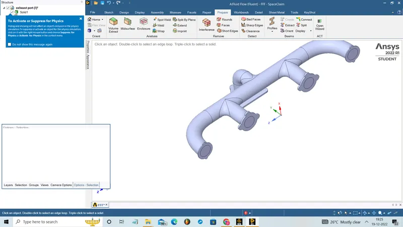
* Select the share tropology option under the workbench which is used to make common node points for two model mesh. So that the information can transfer from one model to other model easily and without any error in data.

* After completing the geomentry open the mesh modul to mesh the model.

* Select the generate mesh option and we wants to change the element size as we wants and considering the number of elements.

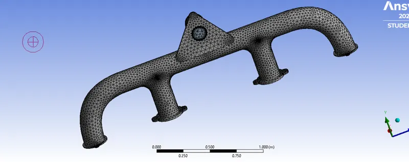
* Assign the name to the models as inlet, oulet, outer wall surface, inner wall surface and fulid volume.

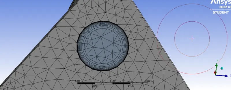
* Create the inflamation layer depends on the Y+ value on the inner fluid volume and bounded with the inner wall surface with

---> first layer thickness = 0.06mm,

---> number of layers =18,

---> Y+ value =1,

---> growth factor =1.3.

* These inflation layer is used to capture the effect changes near to the surface of body close to boundry layer. The inflation layer should be equal or greater than the boundry layer.

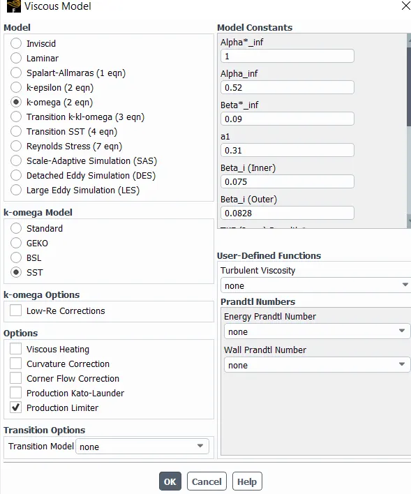
* After the mesh open the set up modul and here we have to set the condition like physics, boundery conditions, type of analysics, Solution setups and the requried outups.

* In these we use the pressure based steady state simulation and Select the realizable K-omega model by opening.

* Enable the enrgy option and Select air as working fluid by clicking the material option and don't change the default density and viscosity.

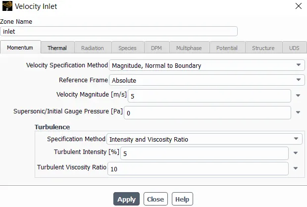
* Then we have to set the boundary conditions by the option boundries . select the inlet and set as 5 m/s and temperature as 700k.

* select the outlet and set as default pressure outlet and set temperature as 300k.

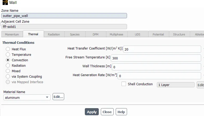
* select the outer wall surface and set to convection and set heat transfer coefficient as 20 W/m^2 K.

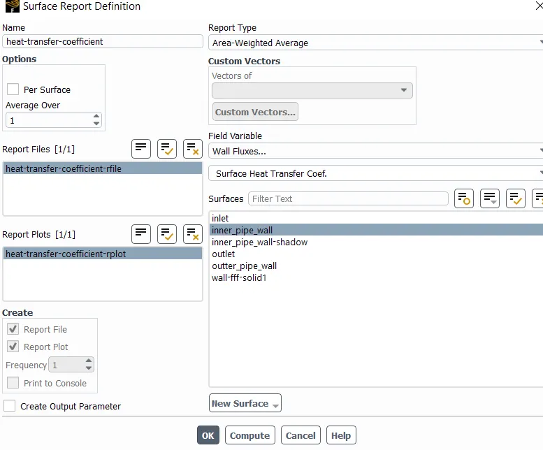
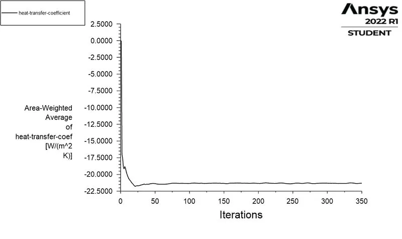
* Then solution set up as to be made to get the Heat transfer coefficient report for inner wall surface by selecting the definition in the solution and select the new and go to Area weight report.

* Select the initialize option to initialize it.

* Give 200 iteration and if the solution is not converged and then increase the iteration and calculate it.

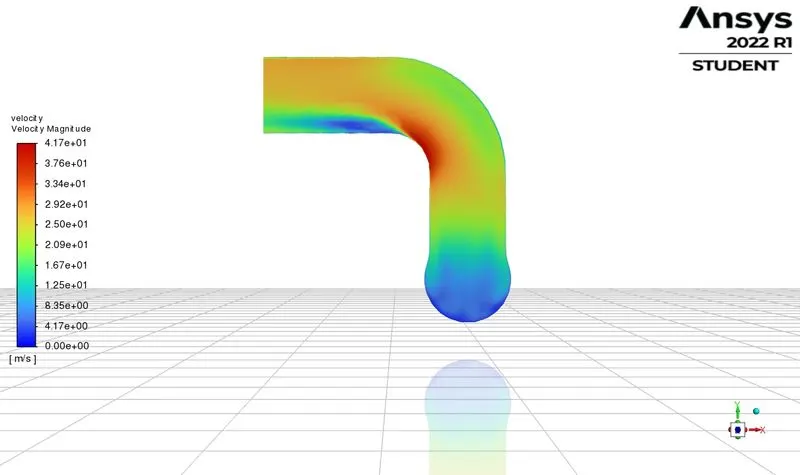
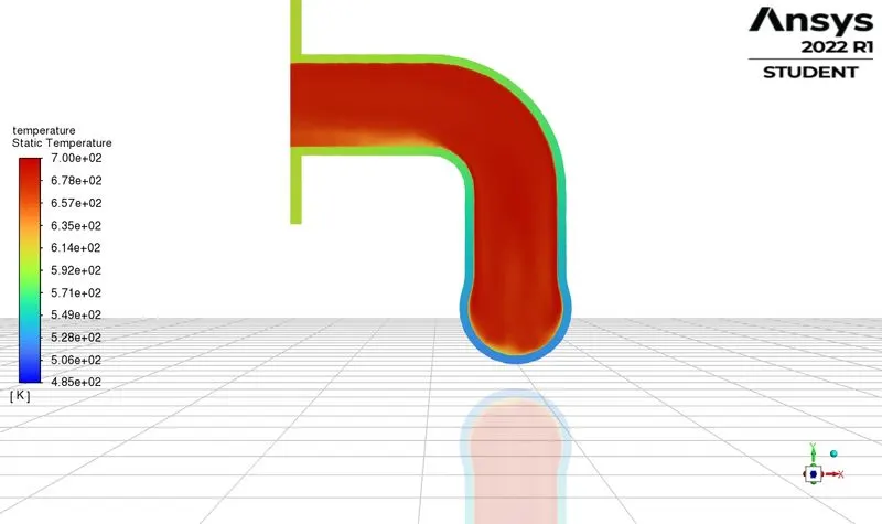
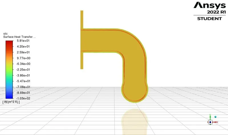
* Create the contours for Temperature, heat transfer coefficient and velocity in the created plane.

* In the result option we can create the plots for Temperature and velocity which is used to compare the results.

RESULTS :

PLOTS AND COUNTOURS :

RESIDUAL PLOT :

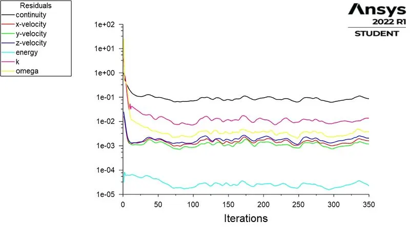
HEAT TRANSFER COEFFICIENT :

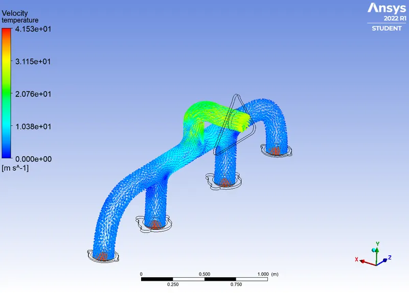
VELOCITY CONTOUR :

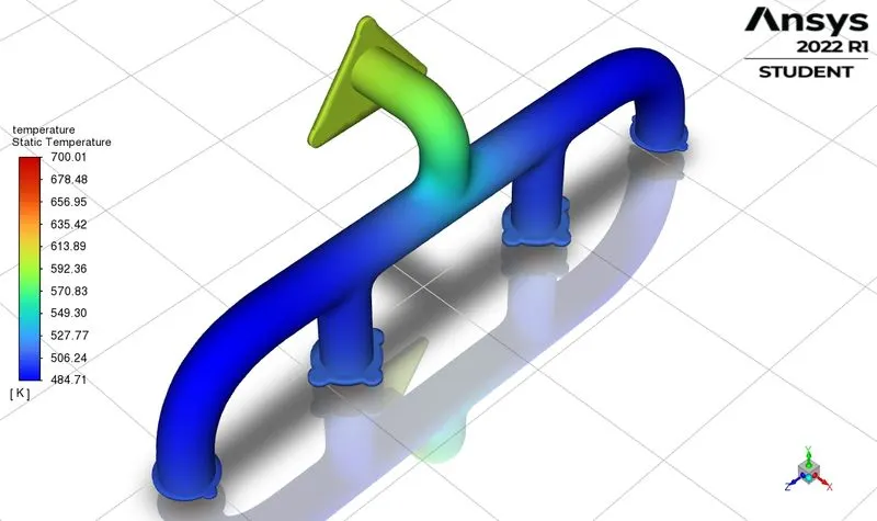
TEMPERATURE CONTOUR :

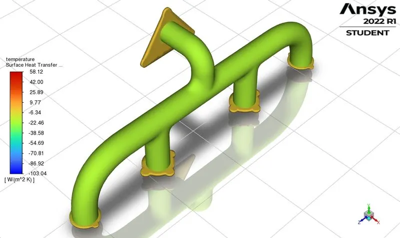
SURFACE HEAT TRANSFER COEFFICIENT CONTOUR :

TEMPERATURE IN PIPE :

SURFACE HEAT TRANSFER COEFFICIENT IN PIPE :

VELOCITY VECTOR :

VERIFICATION :

To verify the HTC predicted value from simulations are right, we can used the analytical method.

Heat transfer coefficient can be determined using the Nusselt Number (Nu) equation,

Nu= convective heat transfer / conductive heat transfer

=h/(k/L) =(h*L)/k

where,

h = convective heat transfer coefficient in W/m^2.K

L = characteristic diamerer in meter = 0.166m

k = thermal conductivity in W/m.K = 0.0242 W/m.K

To determine, Nusselt Number, the Dittus-Boeltr equation for internal turbulent flow condition will be used which is,

`Nu = 0.023 * Re_(Dh)^0.8 * Pr^0.4`

where,

Pr = Prandtl Number for the air with 700 K temperature = 0.71

Re = 56820

So, Nu = 0.023 * (56820)^0.8 * 0.71^0.4

= 127. 59

From first equation of Nusselt Number,

h = (Nu*k)/L = (127.59*0.0242)/0.166

= 18.6 W/m^2.K

So, the heat transfer coefficient consider for the simulation, which is 20 W/m^2.K, is very near by the calculated heat transfer coefficient. The calculated Nusselt Number's value depends on the Prandtle number & Reynolds number. And also, the Dittus-Boeltlr equation is accurate for the smooth circular pipe with small to moderate temperature differences and it is less accurate for rough pipes & large temperature variations. Because of these factors, the difference in the calculated heat transfer coefficient & coefficient consider for simulation is acceptable.

Factors that the accuracy of the prediction depend on :

• The factors that the accuracy of the prediction depend on are
• We need to make sure that share topology is set to share.Only then the meshing is going to be uniform and with perfect connectivity.
• We need to select exact turbulent model.As it is wall bounded flow k- omega SST will be very much suitable.And when selecting the turbulence model selecting exact Y+ value also important.
• We need to give exact heat transfer coefficient for the outer boundary.Then only we get the overall accurate solution.
• While giving the values,like for inflation layers or any other values with decimal values,give the exact values or else it may lead to round off error.
• Since at the interface it is very important as we want to calculate the heat transfer at that place we need to take that region and create inflation layers so that flow is captured exactly and the values are calculated exactly.

CONCLUSION :

A CHT simulation on the exhaust port of an automobile is performed and the wall HTC is determined.