Week 4 - CHT Analysis on Exhaust port

Aim:-

1. Give a brief description of why and where a CHT analysis is used.
2. Maintain the y+ value according to the turbulence model and justify the results.
3. Calculate the wall/surface heat transfer coefficient on the internal solid surface & show the velocity & temperature contours in appropriate areas.
4. How would you verify if the HTC predictions from the simulations are right? On what factors does the accuracy of the prediction depend on?

Give a brief description of why and where a CHT analysis is used.

The Conjugate Heat Transfer (CHT) analysis type allows for the simulation of heat transfer between solid and fluid domains by exchanging thermal energy at the interfaces between them. Typical applications of this analysis type exist as, but are not limited to, the simulation of heat exchangers, cooling of electronic equipment, and general-purpose cooling and heating systems.

CHT analysis type allows for the simulation of the heat transfer between the solid and liquid domains by exchanging thermal energy at the interface between them. The simulation of the heat exchangers, cooling of the electronic equipment, and general-purpose cooling and heating system. In the case of CHT that is being done in this project, we have the convection mode of heat transfer between the fluid and the solid aluminum wall of the exhaust pipe and then the conduction mode of heat transfer is followed within the wall of the exhaust pipe wall.

PROCEDURE:-

(every point is explained in detail below)

1. Geometry
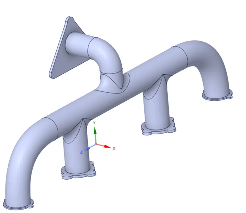
1. Import Exhaust port model in space claim.
2. Extract the volume out of the exhaust port
2. Meshing
1. Set the initial mesh to check every thing is working fine or not.
2. Do the name selection for inlet, outlet, convection wall.
3. Create inflation layer( we will set at the time of mesh refinement)
3. Setup
1. Pressure based solver is used with steady state condition.
2. Energy equation, k-omega viscus model is used.
3. Set the boundary conditions for inlet, outlet, convection wall.
4. Set the contour for temperature.
5. Set a average weighted chart for heat transfer coefficient.
6. Setup the solution animation.
7. Calculate the result.
4. Results
1. Conclusion

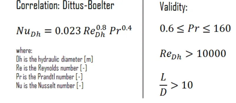
Governing Equation

PROCEDURE Explained .

Ensure first for the unit setup from space claim options.

1. Then import the geometry to the space claim.

Step 2.

we are going to extract volume out of solid body for the calculation purpose.

Prepare>volume extract>select edge and the select the closed edges as shown.

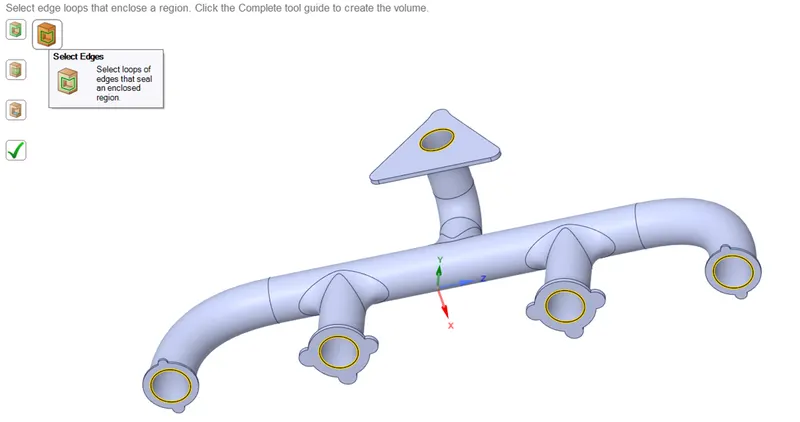
Note= in case of any duplicate edge go to the repair option and select the appropriate command.

Step 3.

Run the meshing to get a feeling that what actually happens.

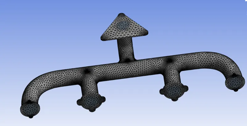
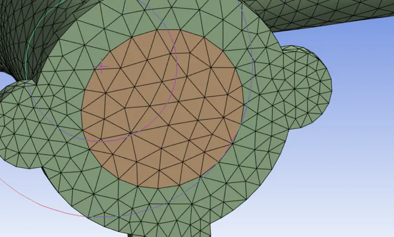
Note:- We can see in the below picture the solid volume and the Liquid volume are not acting as a single body as a result there is non-conformal mesh in this case there is no smooth heat transfer between

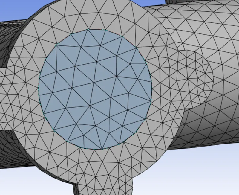
To overcome this we need to close the meshing and in space claim change the property setting to shared topology

But before share topology we need to make solid volume and liquid volume as a same component

For this select both the parts and then right click> Move to new component Re-name the part as final geometry (both solid and fluid volume needs to be in same component)

Then click on FFF and delete empty component.

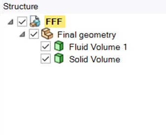
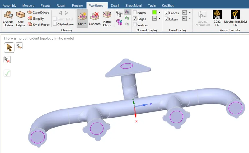
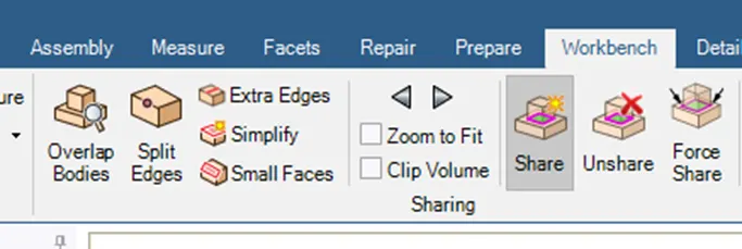
And now go to the workbench tab and click the share icon

The purpose of this step is to share the interface between solid and liquid volume.

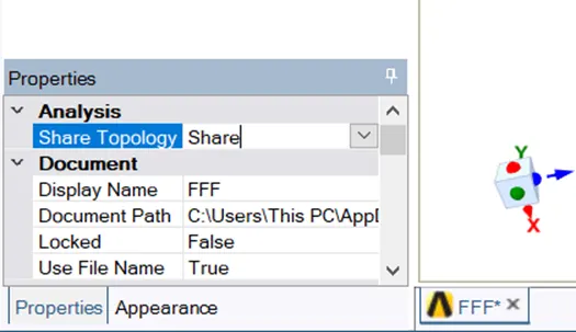
Now change the topology setting to share from None

Then go to workbench (on top of the bar) <share (If we not do this we can not see the interfaces where information have been shared)

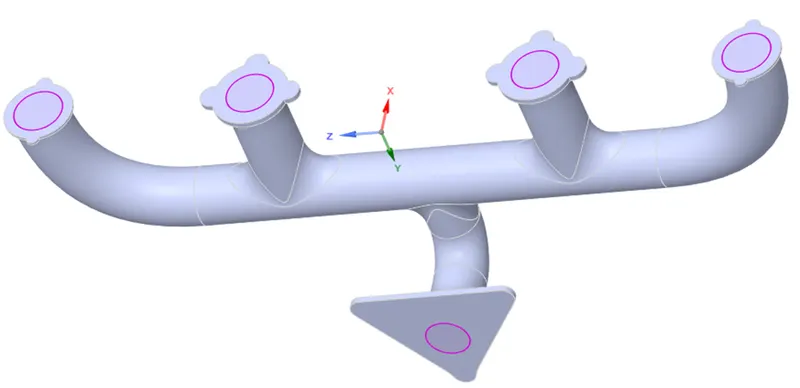
And after this re-run the meshing and we'll see every thing is sorted. (We generate this mesh just to ensure the conformal mesh so, clear generate mesh because we didn't provide the faces name.)

Step 4.

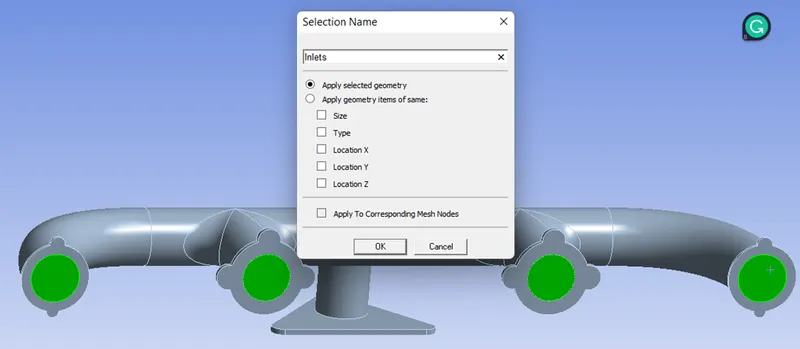
clear the generate the mesh now and select the faces to name them and then hit 'N' and name accordingly.

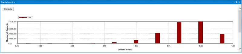
Then again generate mesh and check for the statistics elements and nodes (This case is for before refining).

Element quality check, as we require minimum of 10%.

Step 5.

We will set the inflation layer after running the complete setup during mesh refinement.

Now close the mesh and open up the setup

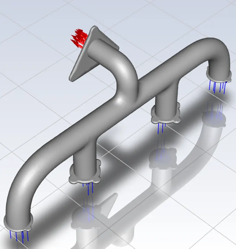
Go to physics on tool bar and Here we are going to define the energy equation

Now set up the project.

Solver type - pressure based solver

State - steady state

Now set up the PHYSICS

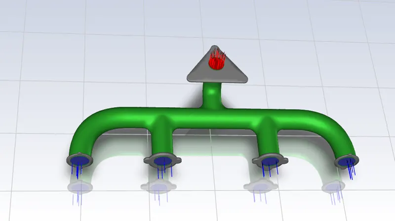
INLET CONDITIONS

1. Initial air velocity at inlet be 5 m/s
2. Temperature be 700k

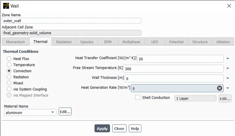
OUTER WALL CONDITION

1. Heat transfer coefficient to 20 w/m^2 k

This value is based on lots of experimental data.

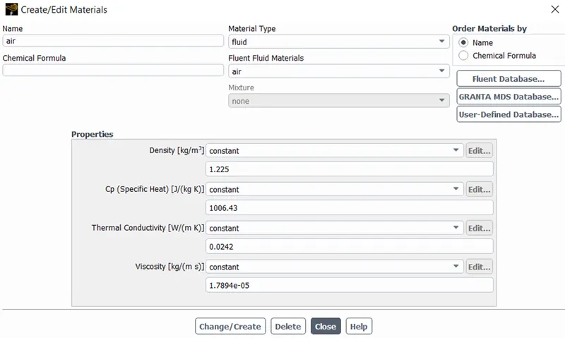
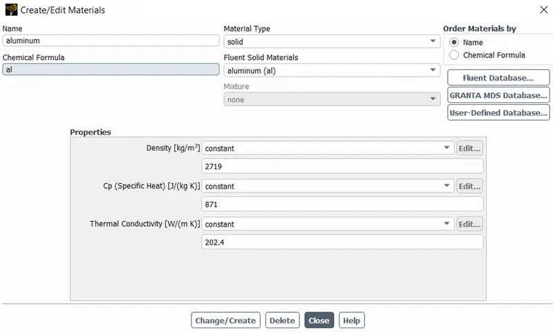
Material Detail

Fluid -Air:-

Solid Material - Aluminum

ENERGY EQUATION

Viscus model > K-omega viscus model

Why K- omega model

Using the k-omega SST turbulent model as it predicts well near walls and combines the benefits of k-epsilon and k-omega,

We need fine meshing near wall and considering the y plus values to be near 5 which falls in the range of k-omega model i.e. 1 to 5

K epsilon is best suited for flow away from the wall, say free surface flow region, whereas k-omega model is best suited for near the wall flow region, where adverse pressure gradient is developed. It's depend on what region of simulation you ahead in near wall is best to use k-w and far wall k-epsilon.

K epsilon is best suited for flow away from the wall, say free surface flow region, whereas k-omega model is best suited for near the wall flow region, where adverse pressure gradient is developed. It's depend on what region of simulation you ahead in near wall is best to use k-w and far wall k-epsilon.

CFD Post

Streamline

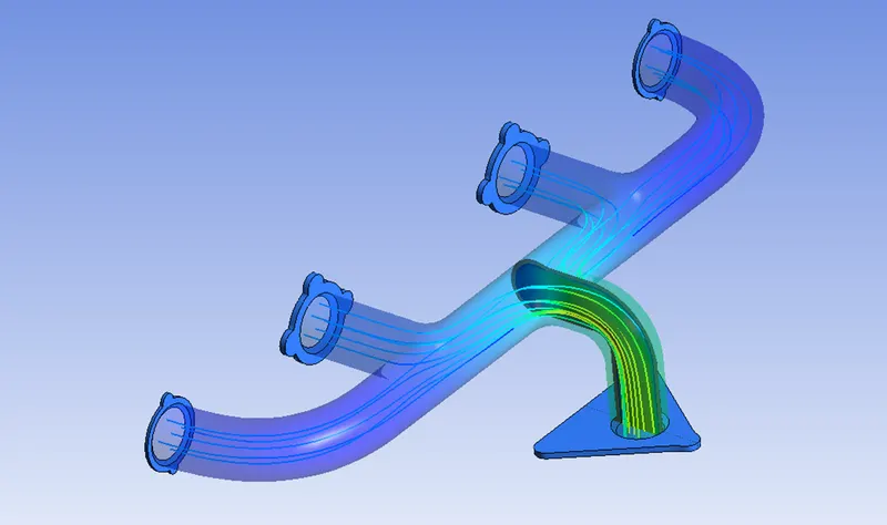
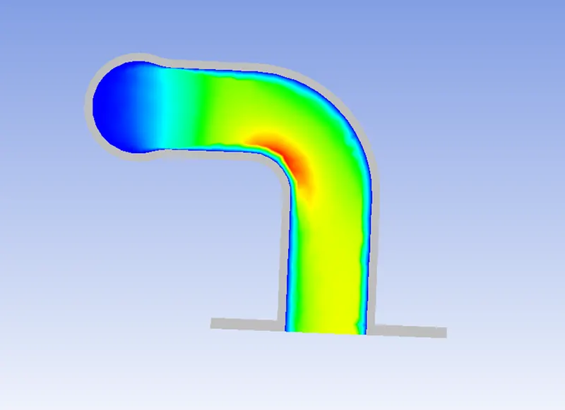
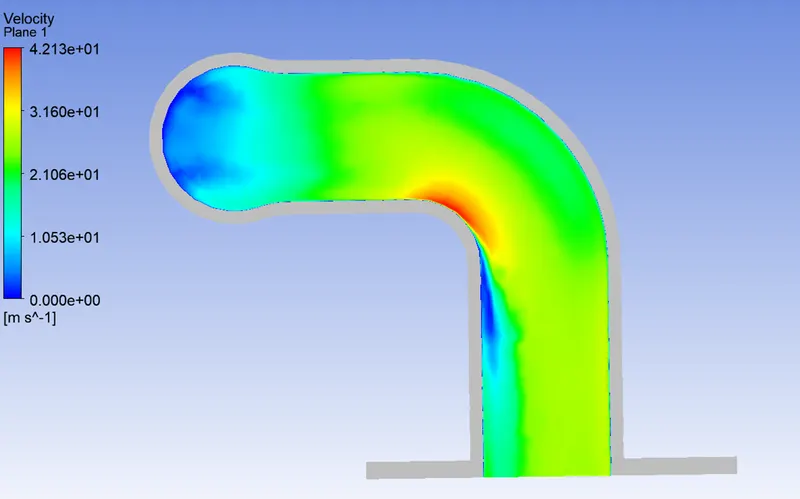
Velocity Contour

Refine Mesh

Refine mesh with inflation layer

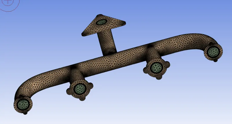
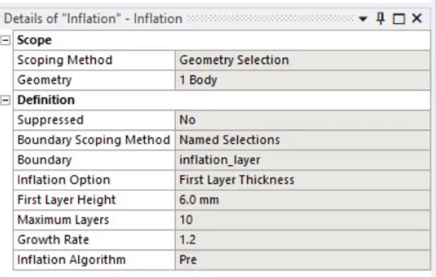
Adding inflation layer

Maintain the y+ value according to the turbulence model and justify the results.

I have used the VOLUPE calculator to calculate first layer thickness.

1. density of air taken from data book for the average temperature of 500 kelvin.
2. Characteristic length is the average diameter of all the pipes.
3. We have taken the k-omega viscus model for which the Y plus is 1-5 so we have taken on higher side.

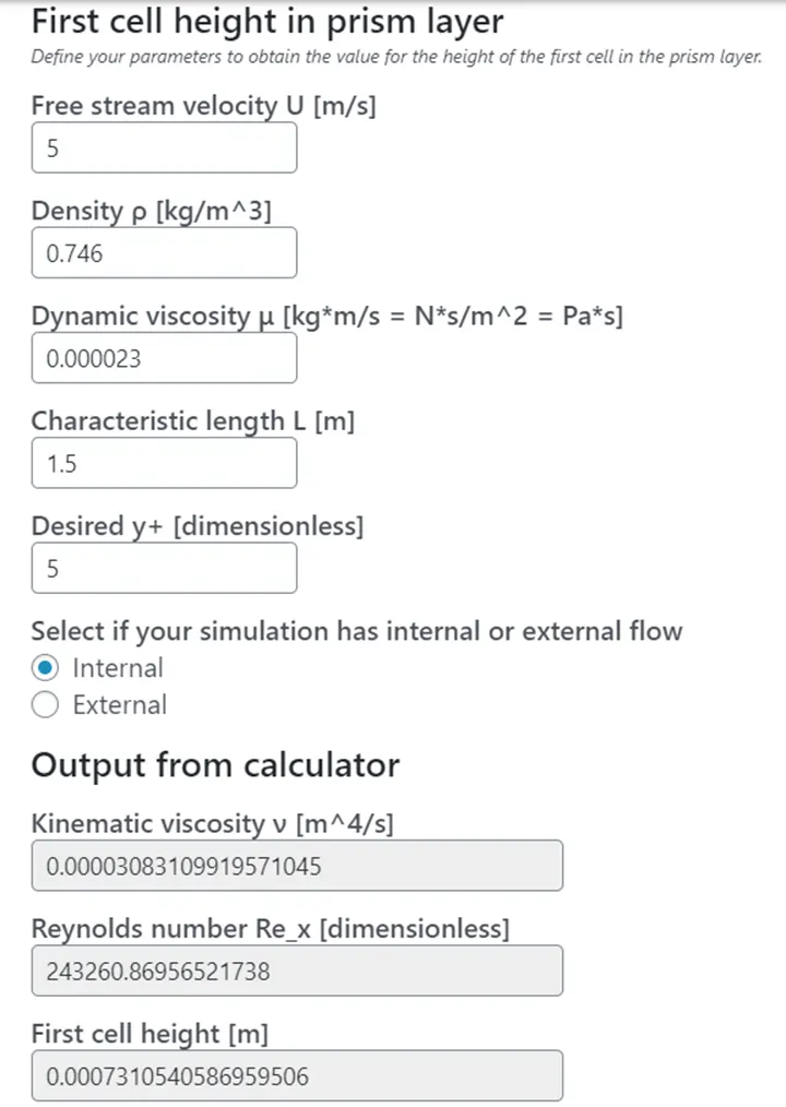
Result the first layer height is 0.7mm

Solution

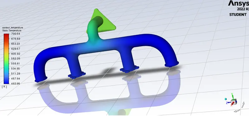
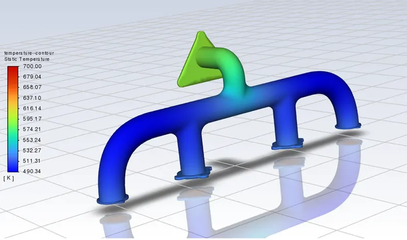
Contour

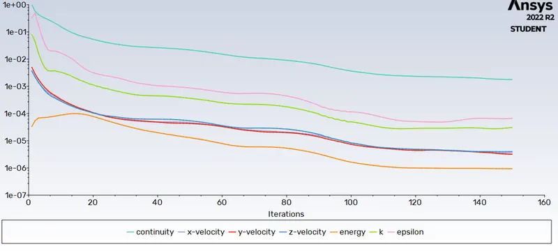
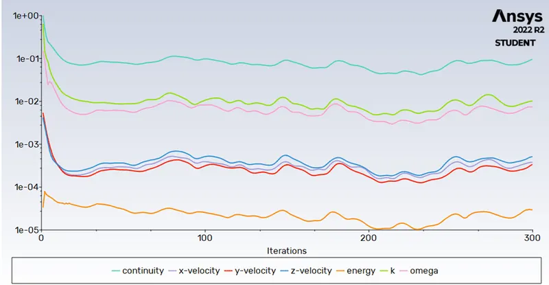
Scaled Residual

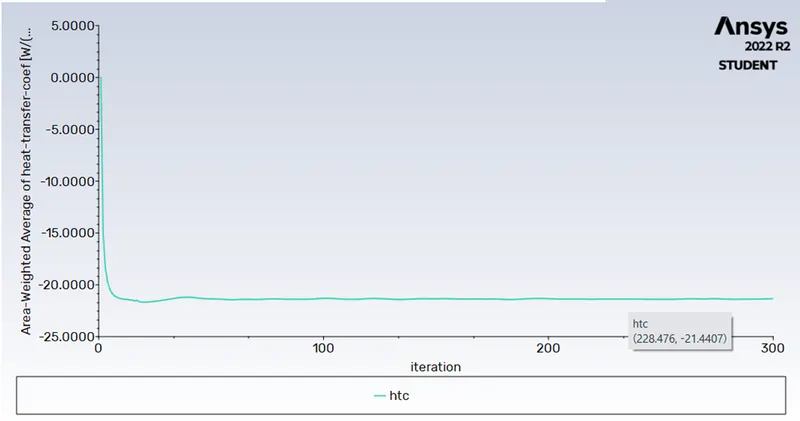
Calculation of the wall/surface heat transfer coefficient on the internal solid surface.

HTC

The value for the heat transfer coefficient is 21.44 Method used coupled

Results

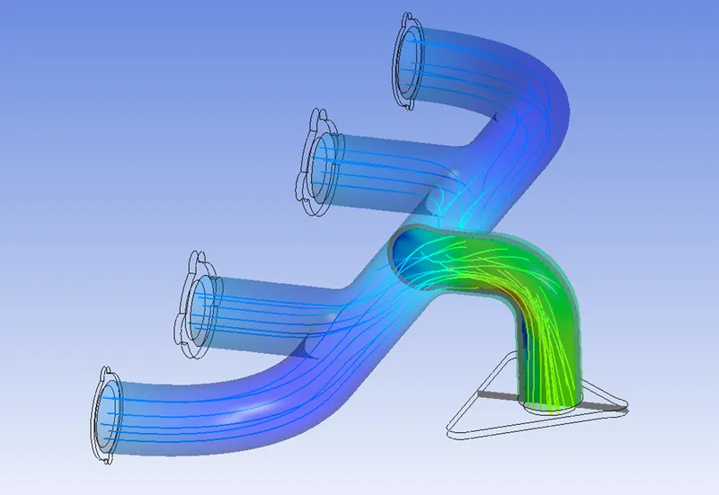
Temperature is much higher at outlet pipe

CONCLUSION

Verification of the HTC predictions from the simulations

In the analysis, the heat transfer coefficient obtained is of h = 21.44 w/m^2-k

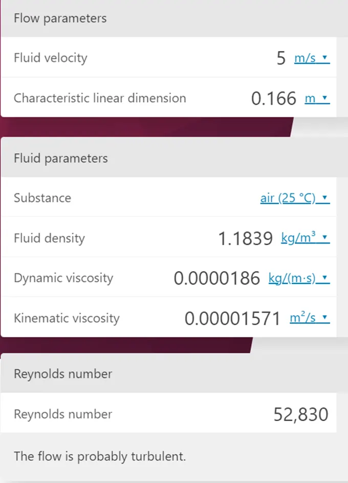
The Reynolds number of the flow is of Re = 52830 considering the flow velocity = 5 m/sec

Pr = mu* cp/k

here mu = 1.789*10^-5 cp = 1006.43 J/kg-k and k = thermal conductivity = 0.0242 w/mk

Pr = 0.00001789*(1006.43/0.0242)

Pr = 0.744

Pr^0.4= 0.888

Putting the values

NU(D)=0.023*52830^0.8 *0.888

NU(D)=122.58

NU(D)=h*D/k

122.58 = h * (0.166/0.0242)

'h = 122.58/6.85

'h =17.89 w/m^2k.

1. Here we find the theoretical value and the computational value of the thermal specific heat transfer coefficient to be = 19.52 so the value is really close to the value of h in the computational way which is = 20 w/m^2k.

2. The value of the y+ is maintained in the range of 5 for the turbulence model . This is validated with the analytical solution which comes out to be near to it. The value of the heat transfer coefficient is found out to be 21.44 w/m^2k. which is close to the analytical value.
3. Because of 4 inlet and 1 outlet the velocity and temperature at outlet is higher.
4. When we are using the finer grid by applying the inflation layer and reducing the element size to be nearly 10 mm we are getting the result with much less deviation.