Week 4 - CHT Analysis on Exhaust port
AIM: CONJUGATE HEAT TRANSFER ANALYSIS ON EHAUST PORT.
> What we are going to do??
We have a solid model of an exhaust port of an inline four cylinder engine and then we are going to modelling the fluid flow through it and solid hest transfer. This is what we called as CHT analysis. Our bjective is to basicaly simulate the flow through port and as the fow is going through manifold it is going to exchange heat with solid we want to simulate heat process also.
> How to do simulation?
We are going to assume that the flow that the flow that is entering in to the exhaust port is very hot and it will heat the solid pipe from inside and in external surfce we are having some particular value of heat transfer coefficient with the help of above setup we can determine the heat transfer rate.
THEORETICAL INRODUCTION:
The Conjugate Heat Transfer (CHT) analysis type allows for the simulation of heat transfer between solid and fluid domains by exchanging thermal energy at the interfaces between them. Typical applications of this analysis type exist as, but are not limited to, the simulation of heat exchangers, cooling of electronic equipment, and general-purpose cooling and heating system.
The term conjugate heat transfer can be used to describe the processes which involve a temperature variation within the solids and fluids themselves due to the thermal interaction between the solid and the fluid.
During CHT the heat transfer can take place from solid media to the fluid media and vice-versa. This is because fluids flow around solids or between solid walls, and also the solids are mostly immersed in a fluid.CHT analysis is beneficial in engineering applications because it shows the heat exchanging capabilities between the two surfaces in the engineering device and various optimization can be done to improve the thermal characteristics of the devices.
Thus, this can be used to improve the heat transfer rate wherever required. It also helps us to identify the key parameters that enhance the fluid flow and heat transfer within the system. Conjugate heat transfer corresponds with the combination of heat transfer in solid and fluid. In solids, conduction often dominates, whereas, in fluids, convection dominates. Efficiently combining heat transfer in fluids and solids is the key to designing effective coolers, heaters, or heat exchangers. Forced convection is the most common way to achieve a high heat transfer rate. In some other applications, the performance is further improved by combining convection with phase change.CHT can be performed to improve the cooling performance of water jackets and increase engine life.
To have analytical or numerical prediction of heat transfer coefficient close to experimentally obtained values, one must focus on conjugating the boundary condition at the fluid–solid interface through coupled heat transfer analysis. Such a coupled field study is termed as Conjugate Heat Transfer (CHT) . However it may be noted that Coupled field analysis is not just limited to CHT studies involving fluidand solid domains. Coupled field analysis or specifically CHT analysis is essential in a situation where solution domainconsists of more than one sub-domains in which heat transfer is governed by different differential equations. In such a case suitable governing equations are to be solved in the respective sub-domains and these solutions need to be conjugated at the interfaces of sub-domains. Aforesaid explicit solution seeking and coupling are also inevitable even if the heat transfer is governed by same setof differential equations, but sub-domains are having dissimilar material properties.
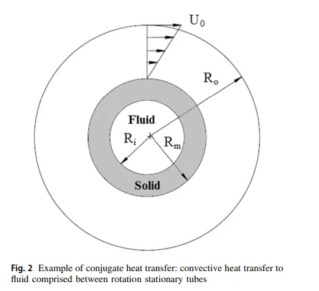
for conjugate heat transfer situation is depicted in Fig. 2. In this case, there is an external tube of outer radius R0, which is heated to a constant wall temperature of 700 K and rotates at constant angular velocity. A fluid field is kept between this rotating tube and a internal stationary hollow cylinder. The internal stationary cylinder is uniformly heated by a hot fluid flowing inside the stationary cylinder. This is a highly conjugated heat transfer situation where two different flow streams and one separate solid domain need to be solved simultaneously to get final solution. This heat transfer setup is very similar to the case of internal cooling of a gas turbine blade.
Advantges:
1. The Conjugate Heat Transfer setup replaces the empirical relation of proportionality of heat flux to temperature difference with heat transfer coefficient. The wall heat transfer coefficients & their local variations are directly computed within the model and do not involve the solving of complex empirical relations. Thus the simulations are carried out much faster.
2. As long as the boundary conditions are accurately defined, the solutions are highly accurate due to the simplicity of the CHT model.
3. There is no limit for the number of surfaces and hence can be applied for a large number of regions in a given assembly.
4. Since the CHT model is a combination of the heat transfers in both a solid & fluid model, it can be applied for all combinations of interactions (i.e. Solid - Fluid interaction, Solid - Solid interaction and Fluid - Fluid interaction)
2) Application of CHT Analysis
CHT analysis is used in various applications to understand the heat transfer between two domains (solid and water or for more than two sub-domain). Some example:-
1. Heat transfer analysis in the cooled turbine blade Wang.
2. Measurement of the heat transfer coefficient in a Channel with Pin Fins.
3. Analysis of a Thermocouple Sensor in a Low-Temperature Nitrogen Gas Ambient.
4. Analysis of Natural Convection and Radiation Heat Transfer from Various Shaped Thin Fin-Arrays Placed on a Horizontal Plate.
5. Conjugate heat transfer and coupled field analysis is aerospace engineering.
6. Conjugate-Heat-Transfer Immersed Boundary Method for Turbine Cooling.
7. Thermal Treatment of Materials.
Exhaust port:
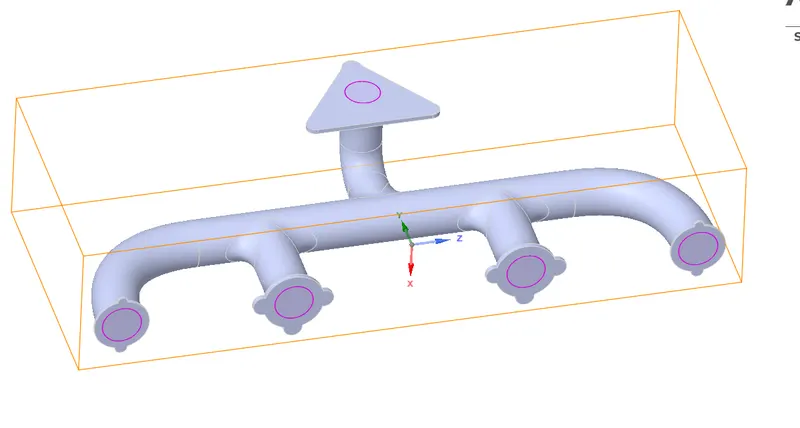
The exhaust port is a three dimensional model containing four inlets and one outlet. Despite having the isothermal boundary condition and a uniform flow rate at the four inlets the model can not be cut into two halves to save computational power. Therefore the whole model needs to be discretized it is also called as space discretization.
Procedure for simulation:
Geometry:
> Importing the geometry.
> Remove extra edges
> Extracting the fluid volume by using volume extract tool
> Sharing the topology by using the share tool which is available in the Workbench.
> Dimensions of the exhaust port.
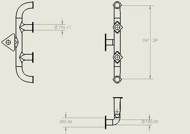
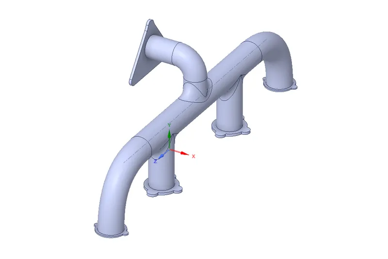
> open spaceclaim and the import the the geometry.
> Eliminate duplicate edges.
select all edges of inlet and outlet but while we are selecting the edges it will not select due to duplicate edge are present.
Repair > Extra edges > duplicate edges are shown by red lines so to eliminate them simply click on them > select green tick symbol so it will delete the remaining extra edges automatically.
NOTE: In complex geometries by simply clicking on the green tick mark it will not eliminate all the extra edges those are present in the geometry so to eliminate all the extra edges sometime we have to select the edges manually.

> Extract the fluid volume.
Prepare > volume extract > select edge option.
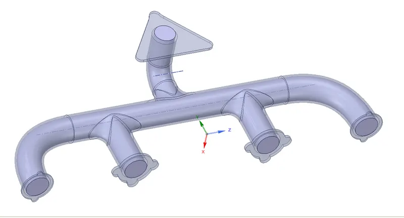
> Select all four inlet and one outlet edge.
Prepare > volume extract > select edges > click on green colour tick mark.
fluid volume will appear.
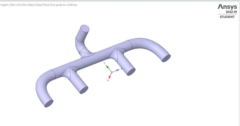
Similarly for solid volume.
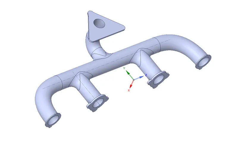
> Give name to the fluid volume.
Prepare > Design1 > Rename volume as fluid volume and solid as solid volume

MESHING:
> Generate mesh with standard element size of 150mm. we assume that the solid and the liquid volume are separate parts in the meshing interface and we have something called as nonconfomal mesh due to which the heat is going to transferred smoothly but in this case this is not happening as there are gap present between the faces at the inlet of the exhaust port.
CASE 1: IN THE FIRST CASE SIMULATION IS PERFORMED ON THE BASIS OF BASE LINE SETUP WITH ELEMENT SIZE OF 150mm without inflation layer.

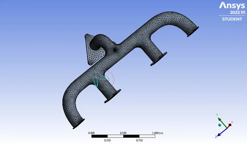
> The heat will not transfer from the interface due to presence of non conformal mesh.
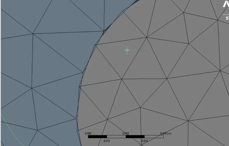
> in order to remove the non conformal mesh use share topology.first delete the mesh and open the geometry..
Workbench > share > click on tick mark.
This share option will take care interfaces so that we only have one interface between solid volume and fluid volume.

click on fff > enable share topology.
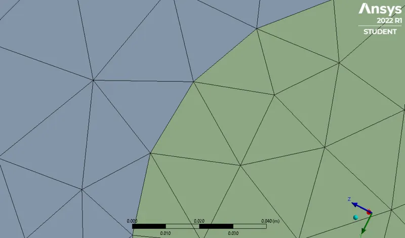
Due to enabling of the share toplogy two interfaces will be shared at the common node points. Spaceclaim gives an option for share coincident topology when share coincident topology is selected and executed. The , mesh from the fluid volume and the solid volume are said to be conformal with each other which is a requirement for the CHT analysis.
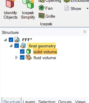
> Create the final name where it comprises both solid and liquid volume and name it as Final geomety.
click on solid component and fluid component together and then right click select move for new component and name it as Final geometry.Now solid component and fluid component ae the empty part. Right click on fff and select DELETE EMPTY COMPONENT.
> Pink circles present at the inlet and outlet pipe reprasents that the interface has been shared.
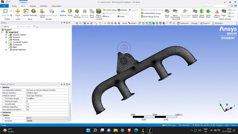
> Close geometry and generate mesh with default element size.
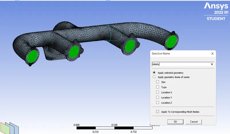
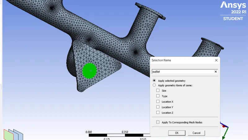
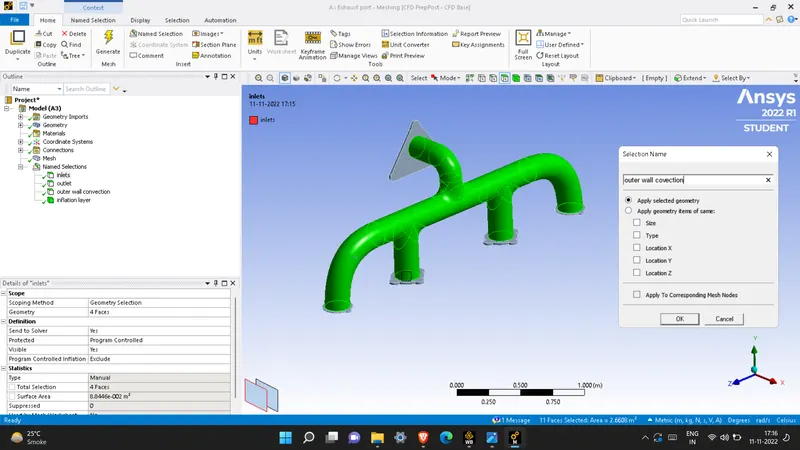
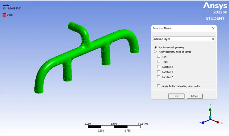
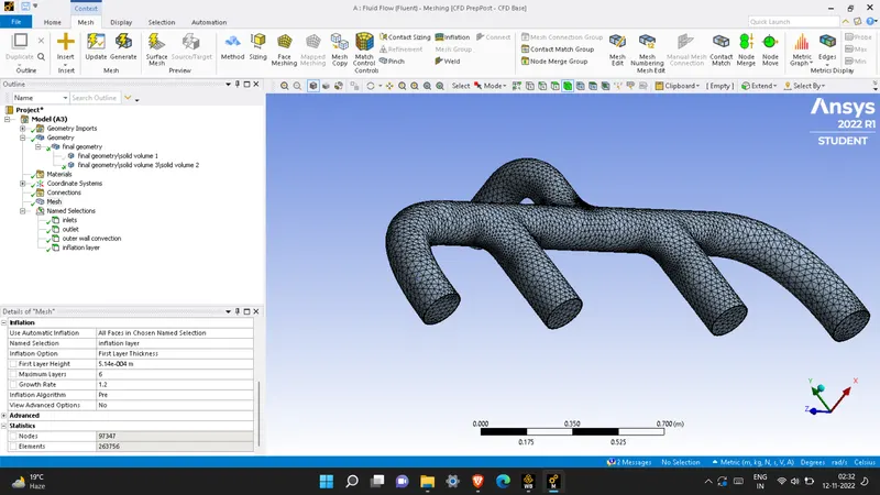
> Give name selection.
Inlet
Outlet
Outer wall convection
inflation layer
> ELEMENT Quality:
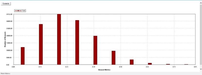
Element quality should not be less than the 10%.
Number of elements as 264698.
> SETUP:
| SOLVER TYPE | PRESSURE BASED |
| SOLVER TIME | STEADY STATE |
| ENERGY | ON |
| TURBULENCE MODEL | K-OMEGA SST |
| MATERIAL |
FLUID- AIR SOLID- ALUMINIUM |
| BOUNDARY CONDITIONS( INLET) | VELOCITY AS 5M/S AND TEMPERATURE AS 700K |
| BOUNDARYCONDITIONS(OUTLET) |
PRESSURE OUTLET( GAUGE PRESSURE =0) |
| OUTER WALL CONVECTION | HEAT TRANFER COEFFICIENT AS 20W/m2k |
| INLET SOLID SURAFCE | WALL BC |
| METHOD | COUPLED |
material properties-
Fluid -
Fluid name = air.
Density = 1.225 kg/m^3
Specific heat = 1006.43 J/kg-k
thermal conductivity = 0.0242 w/m-k
viscosity = 1.789e-5 kg/m-sec.
Solid -
the solid material is of aluminum
Specific heat = 871 J/kg-k .
Thermal conductivity = 20W/m2k
In the setup we have choosen k-omega sst model because in the problem we have calculate the wall heat transfer coefficient which is a near wall parameter and for near wall parameters k- omega sst model will give more accurate result then the k-epsilon model.
> RESULTS:
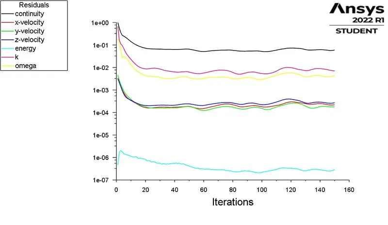
> Scaled Residuals
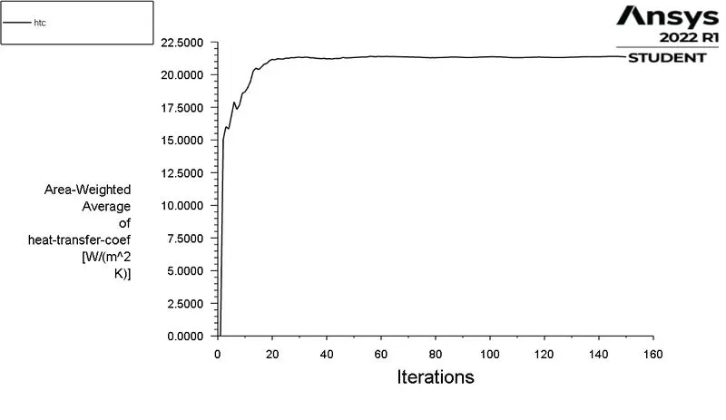
>Heat transfer coefficient:

> Temperature plot:
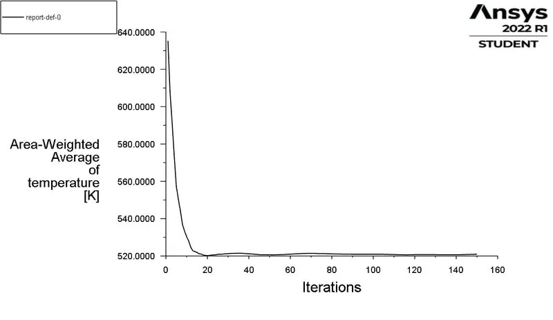
The temperature at the inlet should be highier then the outlet but in this case this shows less the reason for the lower value of temperature at inlet depite being as the hot gases enter in to pipE from inlet is due to convection.
At the outlet fluid has greater velocity then the inlet due to law of conservation of mass as it states for stedy state the mass flow rate at the inlet should be equal to mass flow rate at the outlet and when this is the case that means the velocity at the outlet should be greater than the velocity at inlets for balancing the mass flow rate as we know that
mass flow rate = density of fluid * area * velocity of fluid
Due to highier velocity at the outlet it results in highier value of the heat transfer coefficient as heat transfer coeficient is not a property of the material it is a experimental determine value which depends upon the all the variables influencing convection such as surface geometry , the nature of the fluid motion,the properties of the fluid, and the bulk fluid velocity.
so due to highier value of the heat transfer coefficient at the outlet it results in more rate of heat tranfer from fluid to solid due to more heat passes at the outlet section due to which the Temperature of the outlet section is greter then the inlet section of the exhaust port.
> POST PROCESSING:
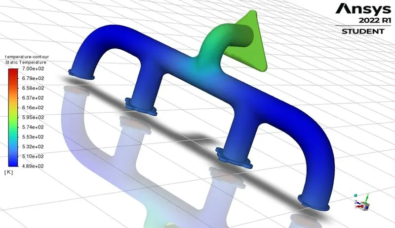
> Temperature Contour at outer wall convection:
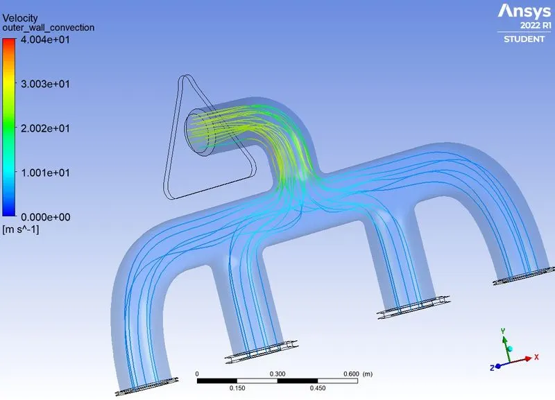
> velocity at outer wall convection:
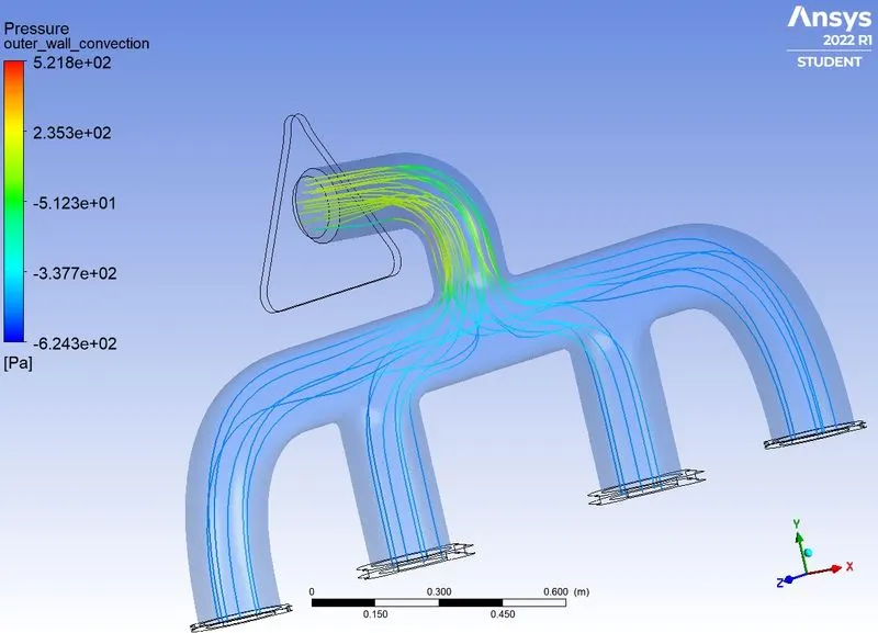
> Pressure at outer wall convection:
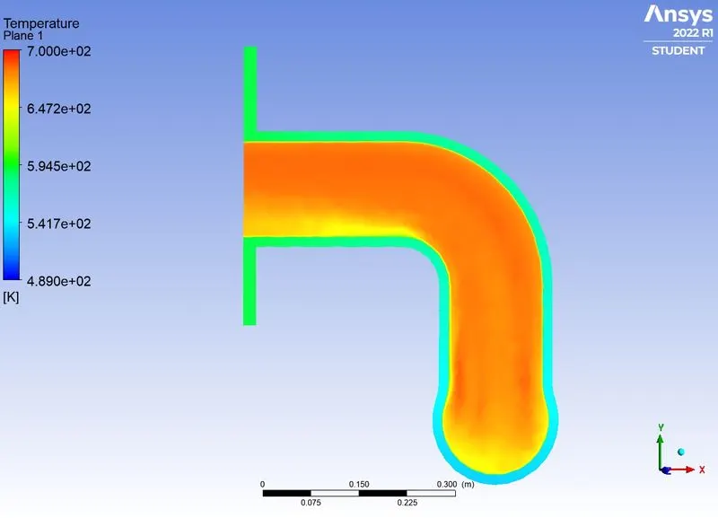
Temperature at xy plane:
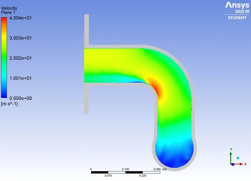
Velocity at xy pplane:
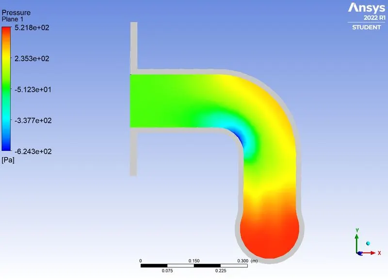
> Pressure contour at xy plane:
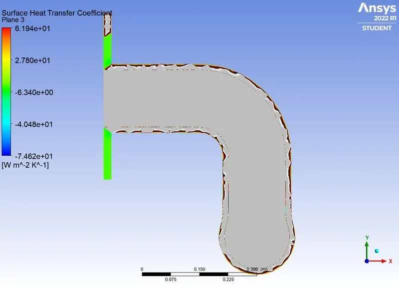
> Surafce heat transfer coefficient at xy plane:
case 2 )
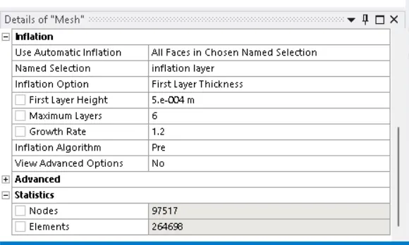
We are going to choose the model to be k-ω and for that Y+ value should be less than 5 so we are going to add inflation layers in the mesh. So for that, we are going to give the inflation layer on the fluid with the first layer thickness to be 1mm with a 20% growth rate and we are going to generate the mesh.
In the next step, we will add the inflation layer to the model. We simply right-click on the Mesh and then add an inflation layer to the Fluid region of the Exhaust port that we created.
Y+ value:
Y+ value is used for calculating the first layer thickness and in this case the first layer thickness is required for get the thickness up to which fine structured mesh has een generated.
To get the thickness up to which fine structured or body fitted structured mesh( inflation layer) is performed we use first layer thickness.
The y+ value is a non-dimensional term that can be used to understand how coarse or fine our grid is. THis can be used to define if the wall fuctions need to be used or not.
Y+ value depends upon the first element. So to get a small Y+ value we need to make our first element very small and to get the Y+ value large we are gonna need the first element to be large. So in this challenge, we are going to use the inflation layer. We are going

where
y = distance from the wall
u_t = frictional velocity
v = kinematic viscosity
We decide what turbulence model we need to choose on the basis of our Y+ value. If the Y+ value is less than 5 it is good to choose the k-ω" model but if the Y+ value is more than 30 we have to use the k-ε model.
`o in this challenge, we are going to use the inflation layer. We are going to use the k-ω model so we have to keep the Y+ value to be less than 5. So keep that in mind we are going to give the first layer to be in that range so that the Y+ value does not go beyond the 5.
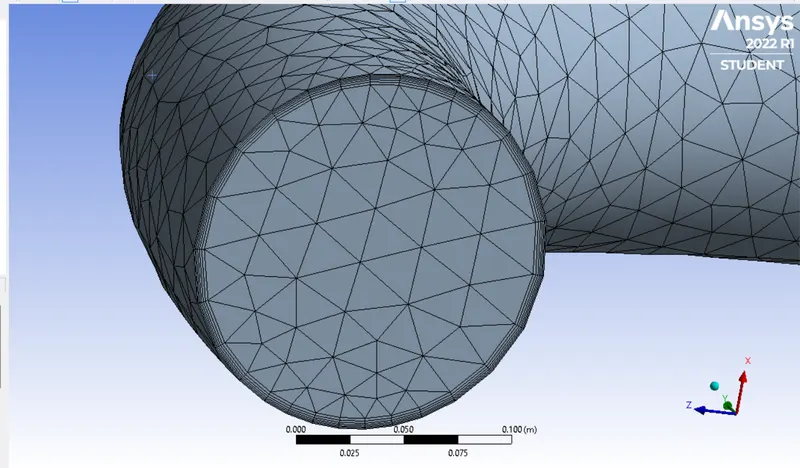
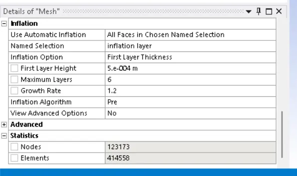
The Inflation layer is added to the geometry 6 layers are added
Growth rate = 1.2
Number of inflation layers = 6
First layer thickness = 0.0514 mm
captured curvature is set to yes.
>Meshing:
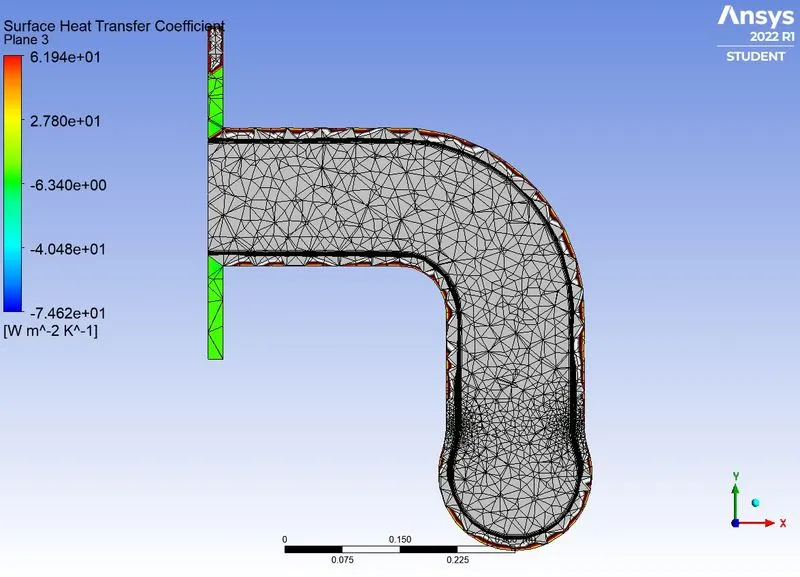
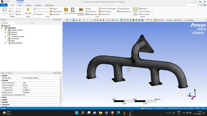
Delete the previous mesh and generate the mesh with element size of 50mm for the outer wall convection and for body sizing (inflation layer) 15mm. here we have less size of element size for inner part becuase we have to calculate the heat transfer coefficient at the inflation layer that is at the inner part.
> Create the meshing with element size of 50mm.
> crete the body sizing with the lement size of 15mm for the inflation layer.
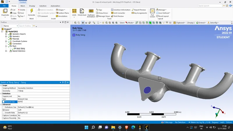
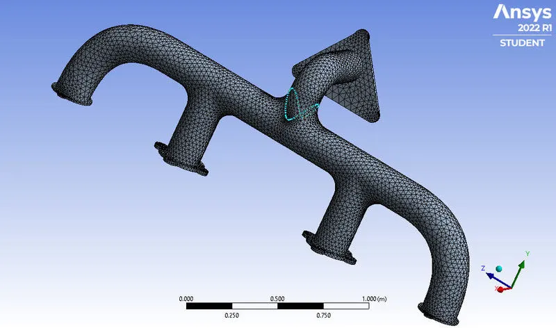
The final meshing will be looks like as shown in below image.
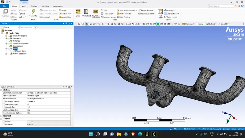
TOTAL NUMBER OF ELEMENTS ARE 414558.
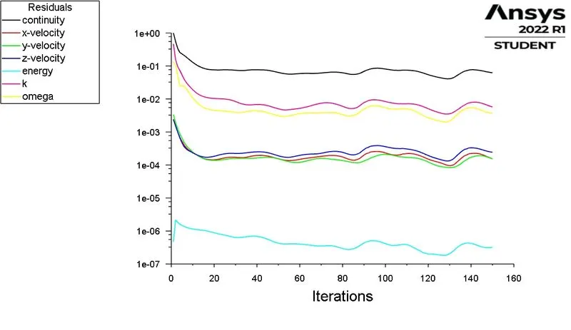
RESULTS:
Scaled residuals:
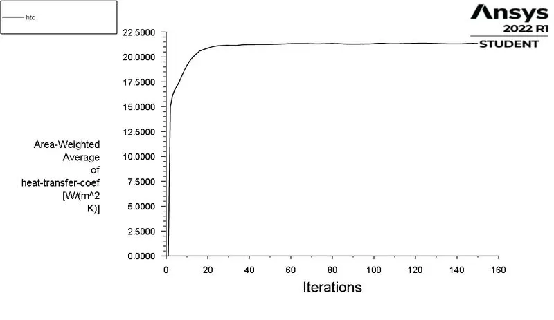
Surface heat transfer coefficient at inflation layer.

> POST PROCESSING:
Temperature contour:
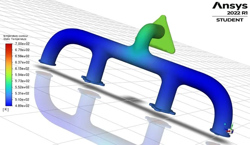
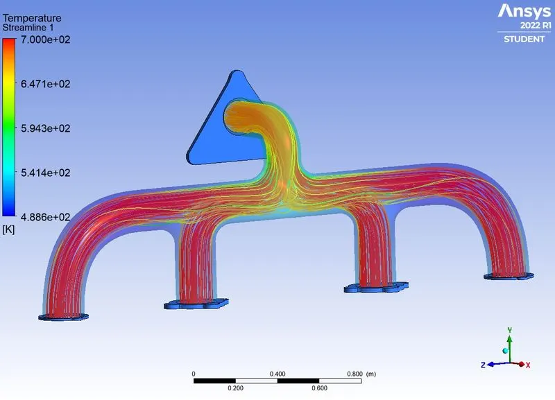
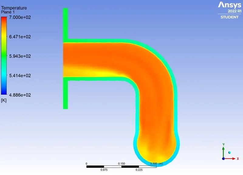
In the above picture, we can see the temperature distribution in the exhaust port. We are getting the maximum temperature at the outlet of the exhaust body. The maximum temperature we got is 700 k and the range of the temperature is 488 to 700 k.
> Velocity contour:
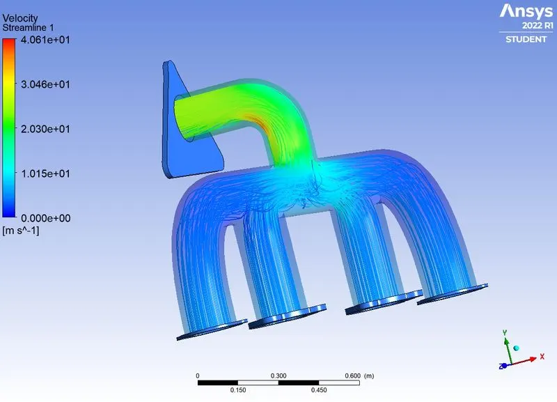
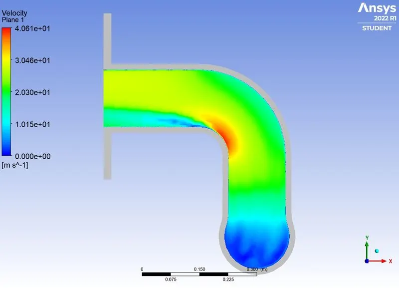
In the above picture we can see that the velocity distribution in the exhaust port. We can see that air is going from inlet to outlet and changing at different points in the port. The maximum velocity we got is 46m/s and the minimum velocity as 0 at the wall of outer wall convection.
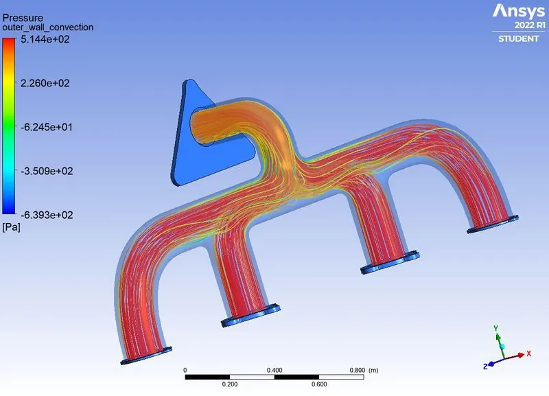
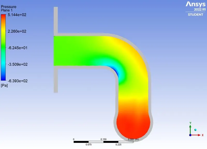
> Pressure contour:
>Temperature contour at xy plane:
> velocity contour at xy plane :
> Pressure contour at xy plane:
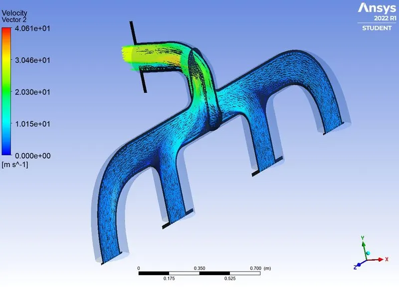
> Velocity vector at diffrent planes:
Velocity vector at two diffrent planes those are xy plane(upward) and yz plane(downward).
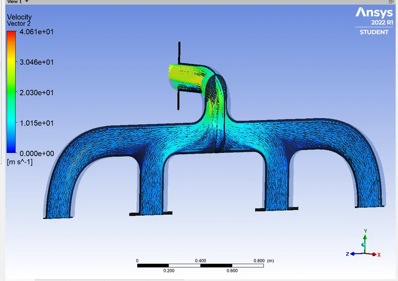
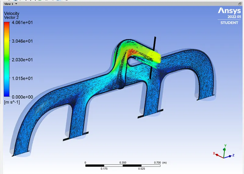
> Surafce heat transfer coefficient at xy plane.
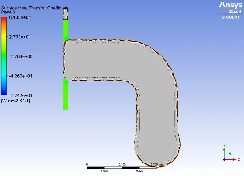
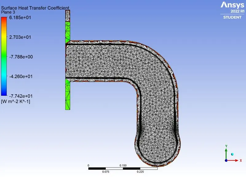
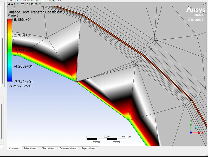
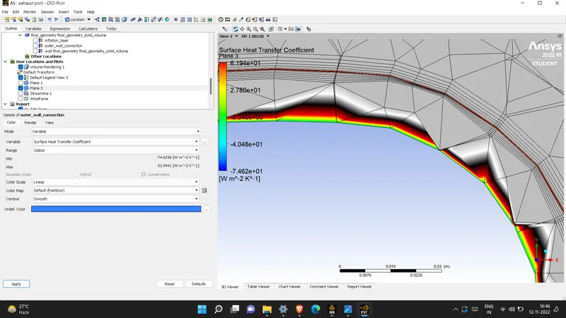
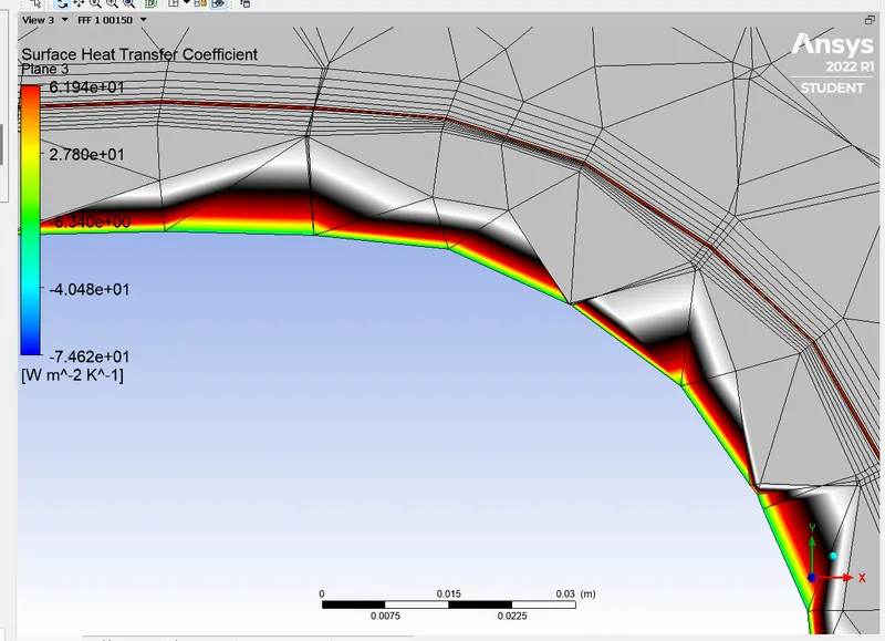
In the above picture we can see the heat transfer coefficient distribution in the xy plane. The maximum heat transfer coefficient value we got is 61.85. The range of the heat transfer coefficient is -77.42 to 61.85
We can see from the above plots that at the bend near the outlet, velocity increases because of that there is an increase of the heat transfer coefficient. We got the maximum heat transfer coefficient there.
> Analytical solution:
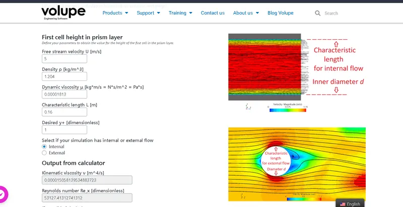
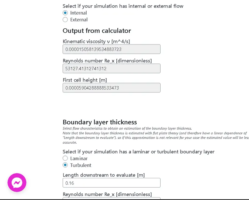
The Reynolds number of the flow is of Re = 53127.41 considering the flow velocity = 5 m/sec
By using the Dittus Bolter heat transfer coefficient relation in natural turbulent internal flow the Diltus Bolter heat transfer coefficient is determined by the Nusselt number which is related by the formula of
Nu(D) = 0.023* Re^(4/5)*pr^n here n = 0.3 . D = diamter of the pipe = characteristics length = 0.166 m, n=0.3 is for cooling of the fluids
the prandtl number is of the following
pr = mu*cp/k here mu = 1.789*10^-5 cp = 1006.43 J/kg-k and k = thermal conductivity = 0.0242 w/mk
pr = (1.789*10^-5*20)/0.0242 = 0.744
the Nusselt number is calculated as NUd = 0.023*56867.66^(4/5)*0.744^0.3 = 131.792
Nud = hD/k = 131.792 = h*0.166/0.0242
so h = 19.52 w/m^2k.
We have use a online calculator for calculating the value of first layer thickness by assuming Y+ value as 5mm.
GRID INDEPENDENCE TEST:
For grid independence, we are going to compare the heat transfer coefficient value for different-different mesh sizes.
| Case | Mesh Size (mm) | No. of Elements | Average Transfer Coefficient in Inflation Layer |
| Case-1 |
Solid Region Mesh Size = 150 Fluid Region Mesh Size = 150 |
264698 | 21.359 |
| Case-2 |
Solid Region Mesh Size = 50 Fluid Region Mesh Size = 15 |
414558 | 21.340 |
>Conclusion:
Factors that affect the quality of prediction:
- More refined mesh leads to better results.
- Use inflation layers and apply proper Boundary conditions.
- Proper selection of turbulence model according to y+ values.
> So From the above table, we can see that the value of heat transfer coefficient for different mesh size are almost equal. There is a small deviation in the values and we can conlude that the simulation we have done is right. The grid independence test is a parameter for checking if the simulation we have done is appropriate. The deviation is very less, approximately less than 1% hence we can say that it passes the grid independence test.
> There is no experimental data for this simulation so we can validate by the grid independence test.
> Heat transfer coefficient depends on the area (geometry), temperature, heat transfer rate, the velocity of the fluid and thermal properties of the fluid. Hence, we must be cautious before performing the simulation and check these values.
> When air coming from two ways meet, the air velocity increases, and temperature increases in the solid body. Because of that the heat transfer coefficient is also increases in the solid body.
> From the above cases output, we can say that the results are almost the same but the refined mesh gives us more smoothness and accuracy.
> Two factors influence the performance simultaneously: (a) Flow is developing along the length and the heat transfer coefficients tend to increase from inlet to outlet up to certain length then it decreses
along with flow (b) Turbulence
> At the same time, turbulence is developing with tube rows at the bent, which would increase heat transfer coefficients.
> The maximum heat transfer results at the bend of exit port, It is because to ensure the conservation of mass at exit port velocity should more, which results in higher velocity and increase in velocity attain a Reynolds number that is sufficient to make flow turbulent and higher Nusselt number at pipe bent at the exit, which increases Heat transfer co-efficient at that location.
> The internal flow velocity and its characteristics are affected by the Initial velocity, Pressure, the physical features of the geometry, etc. that affect the heat transfer rates, and hence CHT analysis is essential prior to experimental analysis for better prediction life of the designed component.
> As shown in the plots, the hot exhaust gases passing through the manifold transfer some of the heat to it via convection. The amount of heat transfer can be related directly to the velocity of the exhaust. The temperature is lower where the flow is stagnating or is moving at the inlet velocity. As the velocity increases, so does the Reynolds number and hence the amount of heat transferred..