Week 4 - CHT Analysis on Exhaust port
Aim:
To perform the steady-state conjugate heat transfer simulation on the exhaust port when the air is coming at the inlet at a speed of 5m/sec.
Objective: The objectives will mainly focus on
Give a brief description of why and where a CHT analysis is used.
Maintain the y+ value according to the turbulence model and justify the results.
Calculate the wall/surface heat transfer coefficient on the internal solid surface & show the velocity & temperature contours in appropriate areas.
How would you verify if the HTC predictions from the simulations are right? On what factors does the accuracy of the prediction depend?
Theory:
Heat Transfer by Solids and Fluids
Heat Transfer in a Solid
In most cases, heat transfer in solids, if only due to conduction, is described by Fourier’s law defining the conductive heat flux, q, proportional to the temperature gradient.
For a time-dependent problem, the temperature field in an immobile solid verifies the following form of the heat equation.
Heat Transfer in a Fluid
Due to the fluid motion, three contributions to the heat equation are included:
The transport of fluid implies energy transport too, which appears in the heat equation as the convective contribution. Depending on the thermal properties of the fluid and the flow regime, either the convective or the conductive heat transfer can dominate.
The viscous effects of the fluid flow produce fluid heating. This term is often neglected, nevertheless, its contribution is noticeable for fast flow in viscous fluids.
As soon as a fluid density is temperature-dependent, a pressure work term contributes to the heat equation. This accounts for the well-known effect that, for example, compressing air produces heat.
Conjugate Heat Transfer
Conjugate heat transfer corresponds with the combination of heat transfer in solids and heat transfer in fluids. In solids, conduction often dominates whereas, in fluids, convection usually dominates.
In simple words, it is the heat transfer between solid and fluid simultaneously. There is a thermal coupling at the interfaces of the two regions.
Conjugate heat transfer is observed in many situations. For example, heat sinks are optimized to combine heat transfer by conduction in the heat sink with the convection in the surrounding fluid.
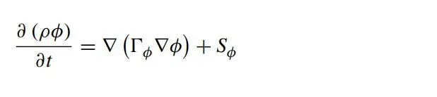
The general form for fluid flow, heat, and mass transport in the fluid (air or liquid) duct can be expressed by

Where t is time (s), ρ is fluid density (kg)/m^3, φ is a general variable which can be velocity, temperature, or concentration, U is the velocity vector matrix, Gamma_phi is generalized diffusivity, and S_phi is a generalized source term. Function div is divergence, and grad is the gradient vector. It can also be expressed as

If Gamma_phi is a constant, then

Where nabla^2 is the Laplace operator.
For ducts in heat and mass exchangers, the solid walls are usually too dense to form a macroscopic fluid flow inside. So the macroscopic fluid flow in the solid is ignored. Heat and mass diffusion in the solid can be expressed in a general form as
Understanding of the complex heat transfer mechanisms and the interactions between those mechanisms to improve the performance and increase the lifespan of the components to be analyzed. Conjugate Heat Transfer analysis provides the temperature distribution in solids and fluids, and clear insight into velocity distribution and mechanism of heat transfer of fluid, like in engines. It is more accurate and fast to simulate the problem. Can be used in complex scenarios like in automotive components or in power plant components.
Multiple regions can be simulated. All types of region combinations can be simulated like solid-fluid,fluid-fluid, etc.
Conjugate heat transfer analysis is based on a mathematically structured problem, which describes the heat transfer between a body and a fluid flowing over or inside it as a result of interaction between two objects. At the matching interface, the details are provided for temperature distribution and heat flux along the interface eliminating the need of calculating the heat transfer coefficient. Moreover, the heat transfer coefficient can be calculated later.
One of the simplest ways to realize conjugation is through numerical methods. The boundary condition for the fluid and solid interface is set and solved through iteration methods. There are no right guesses for the values of the initial boundary condition for the convergence except through the hit and trial method.
Application
The conjugate heat transfer methods have become a more powerful tool for modeling and investigating natural phenomena and engineering systems in different areas ranging from aerospace and nuclear reactors to thermal goods treatment and food processing from the complex procedures in medicines to ocean thermal interaction in metrology.
CHT in recent years has significantly improved the cooling performance of electronic equipment such as the design of heat sinks and the design of heat exchangers for the waste treatment plant. One such application of CHT is the exhaust port system.
Internal Combustion Engines
The internal combustion engine industry is moving toward simulating the entire system rather than independent components. The accuracy of the predicted combustion in the cylinder is dependent on the temperature boundary conditions in the cylinder. By considering heat transfer in the metal components (e.g., the cylinder head, liner, piston, etc.), the cylinder wall no longer has a user-specified temperature. Instead, it has temperatures predicted as part of the complete-system simulation. This makes the overall simulation results more predictive by reducing the dependence on assumed boundary conditions.
Electromobility
Effective cooling strategies are critical for various components of mobility systems. Electric motors have high power densities and thus generate a significant amount of heat. If a motor is not properly cooled, high temperatures in the motor can cause the demagnetization of the permanent magnets and the breakdown of the winding insulation.
After treatment
Predicting and mitigating urea deposit formation is a key challenge in Urea/SCR after-treatment systems. When the urea-water solution is sprayed into the engine exhaust system, it impinges on the wall as a liquid film. The decomposition of urea and the formation of undesirable deposits are highly dependent on wall temperature, and the heat transfer between the film and the wall is important to capture. Predicting the wall temperature helps you identify areas that are vulnerable to wall deposition.
Pumps and Compressors
Resolving the spatially varying surface temperature distributions in pumps and compressors improves the accuracy of the simulation and provides useful temperature data. For example, in a twin screw compressor, thermal expansion affects the clearance between the rotors. If that effect is not captured, the simulations will incorrectly predict leakage flows and lower the accuracy of your results.
In most cases, heat transfer in fluids, if only due to convection, is described by Newton's law of cooling. The Conjugate Heat transfer corresponds with the combination of heat transfer in solids and heat transfer in fluids. Conjugate Heat Transfer Applications: 1) Heat exchanger - It exchanges heat from one fluid to another. Forced convection is the most common way to achieve a high heat transfer coefficient. The separation layers are made of solid. The conduction occurs through the separation layer. (2) Thermal insulators (eg. Polyurethane foam) - Polyurethane foam contains cavities of air which gives the insulation property to the material. (3) Heat sink - It dissipates the heat from electronic devices through convection. (4) Exhaust port manifold - It transfers the burned air mixture from all cylinders to the exhaust system. the solid part of the manifold takes heat from hot gas through convection. then the heat is conducted through the solid part of the manifold. Finally, the heat dissipated through the outer surface of the manifold.
Heat transfer coefficient (h):
The heat transfer coefficient, in Thermodynamics, is the proportionality constant between the heat flux and the thermodynamic driving force for the flow of heat.
The heat transfer rate is:
Q = hA (T2 - T1)
Where,
A = Surface area where the heat transfer takes place (m^2)
T2 = Temperature of the surrounding fluid (K)
T1 = Temperature of the solid surface (K)
Wall Heat Transfer Coefficient and Y+ value:
Wall HTC is a quantity that can be calculated at the first cell layer of the wall adjacent to that of fluid.
With the inflation layer, the user can notice accurate capturing of Wall HTC along the surface separating solid and fluid volumes.
Maximum HTC is predicted/captured at the same location of maximum velocity.
Solving and modelling approach:
In this study, we are going to analyze the heat interaction between the exhaust manifold and the fluid flowing in it. For this, we will use two different meshes and generate temperature contours also. Another setting is going to same. The following procedure is followed to analyze CHT on the exhaust manifold.
Case 1
The exhaust port is a three-dimensional model containing four inlets and one outlet. Despite having the isothermal boundary condition and a uniform flow rate at the four inlets the model can not be cut into two halves to save computational power. Therefore the whole model needs to be discretized it is also called space discretization.
CHT analysis requires both the solid and the liquid volume under consideration Spaceclaim gives an option of volume extract for selecting the edges for fluid volume.
Both the solid component and the liquid component are copied into one component.
Share topology is created.
Spaceclaim gives an option for share coincident topology when share coincident topology is selected and executed. Then, the mesh from the fluid volume and the solid volume are said to be conformal with each other which is a requirement for the CHT analysis.
The exhaust port is loaded with the proper geometry and it is then simulated for the baseline computer-generated mesh in the next half we are going to be when we are going to use the refined mesh using the inflation layer and the element size is to be updated to 25 mm and hence a finer result is obtained.
The named selection is created like the inlet one, outlet one, and the outlet and the wall-convection are created to study the effect of convection from the fluid to the wall and from the wall, the heat is dissipated by the heat conduction method.
Geometry preparation:
Import the geometry to the space claim from the step file format.
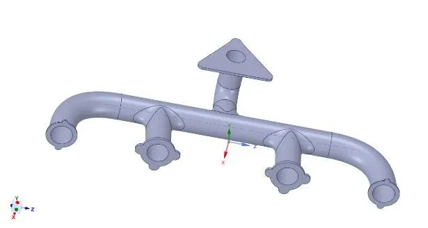
Inside the SpaceClaim, the extra edges were found in the geometry that was provided we have to remove them by the option of prepare, and the six edges were removed.
Then the volume extraction tool is used for the five edges and volume and the process of fluid volume extraction is used for the edges to create the fluid volume.
Prepare the geometry for extracting the fluid volume from the solid domain. To do that go to prepare physics. Click on volume extraction.
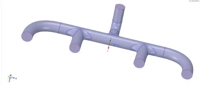
Select the inlet edges and outlet edges of the exhaust port.
Now move the solid and fluid domain to a new component.
This is obtained by right click on the work tree diagram and select move to the new component.
Go to the workbench, and select the share prep option. After the topological sharing will be completed, the entire internal region will be highlighted in red. The external edges of the inlet and outlet will appear pink.
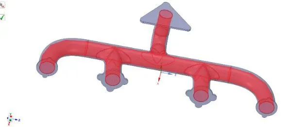
Once topology, sharing is completed, the final geometry preparation is completed.
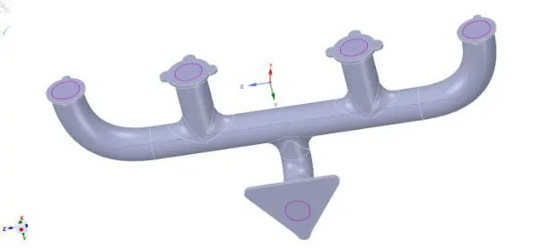
Conformal meshing is performed to share the topology at the solid and fluid domains successfully. Without conformality, the meshing interface would cause a lot of interpolation at the boundaries which could eventually lead to improper meshing and non-uniform heat conduction at the boundary zone. This may confirm the smoothness in grading at the fluid domain due to the wall y+ effect.
Meshing:
Open the meshing console.
Once the geometry is opened, select mesh and click generate.
A normal basic mesh will be created.
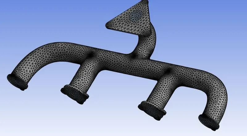
Now refining the mesh.
Before refining, we create the named section to certain geometrical parts.
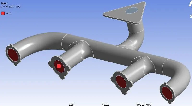
Select the inlet faces of the exhaust port as the inlet.
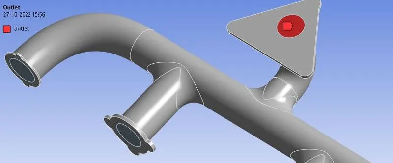
Select the outer faces as outlets.
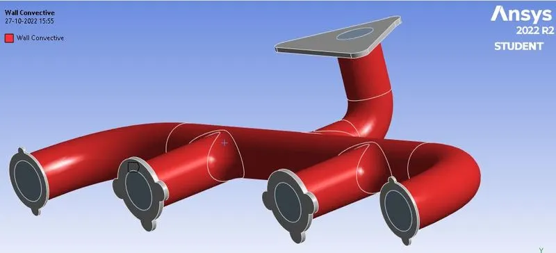
Select the body of the exhaust port and define it as wall convective.
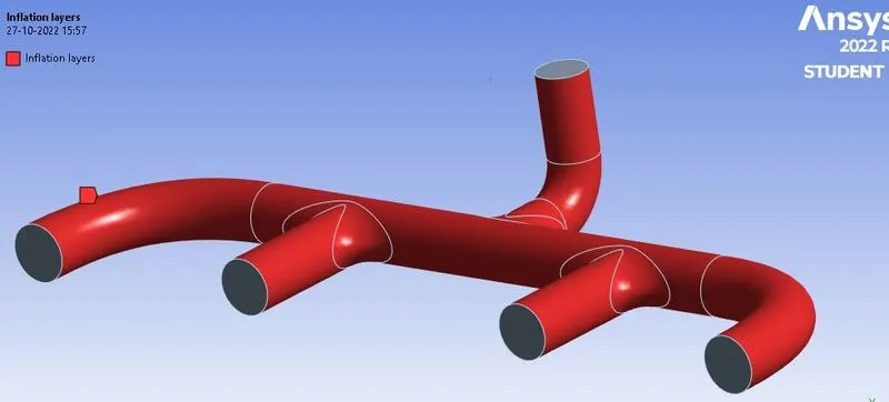
Select the inner fluid domain and name it inflation layers.
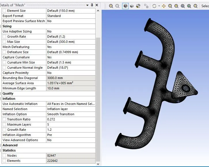
Baseline mesh setup
Nodes: 82447
Elements: 222642
Default Mesh size: 150 mm
The baseline mesh is created due to the original geometry with fewer modifications.
Then it is imported into the fluent solver to perform the CHT flow heat transfer analysis.
Solver setup
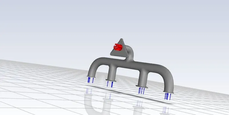
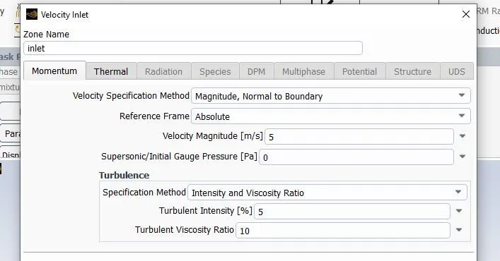
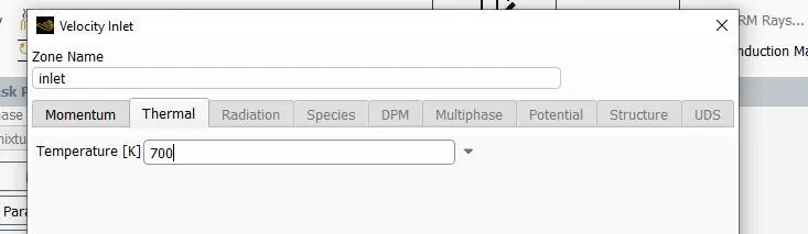
The following inputs of the variable are made into the following velocity v = 5 m/sec at the inlet with the temperature of the fluid to be 700 kelvins. The boundary condition applied at the inlet is of velocity inlet.
The red arrow indicates the outlet the boundary condition is of the pressure outlet type. The third boundary condition is applied to the outer wall convective with a heat transfer coefficient of k = 20 w/m^2-k.
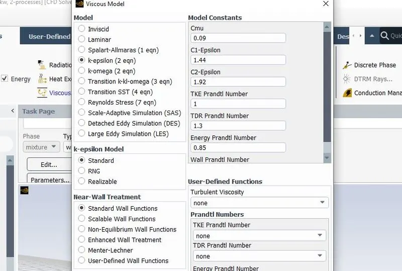
The steady-state pressure-based solver is used with the Coupled algorithm and the turbulence model that is used of the k- epsilon turbulence model is used with the outlet Gauge pressure = 0 pa and the energy equation is turned on.
Viscous Model
Inlet conditions
In this problem, the temperature of the inlet port is important so the temperature field is activated. The second step is to define the material, where fluid is taken as air and the solid domain is taken as aluminum. Setting up the cell zone boundary conditions, we define the solid domain and fluid domain. The third step is to give the inlet of the exhaust manifold a velocity of 5 m/s and an inlet temperature of 700k.
Wall convective conditions
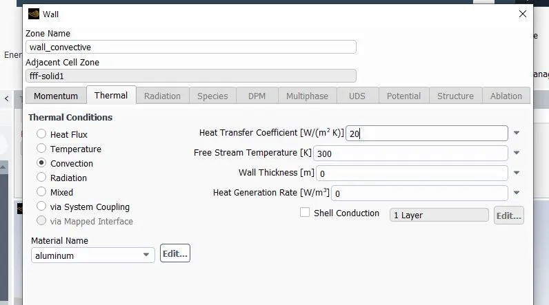
The outlet is kept as a pressure outlet and the outer wall convection is defined with a heat transfer coefficient of 20w/m^2-k. the other walls are kept as isothermal.
Material properties
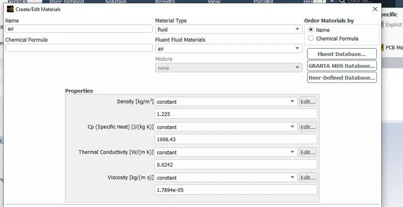
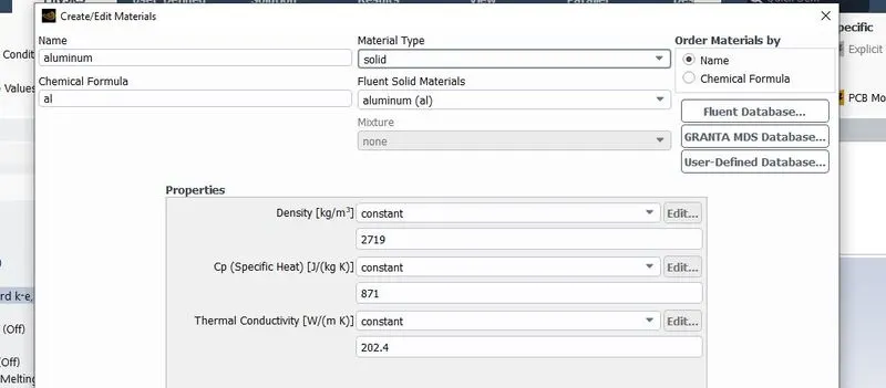

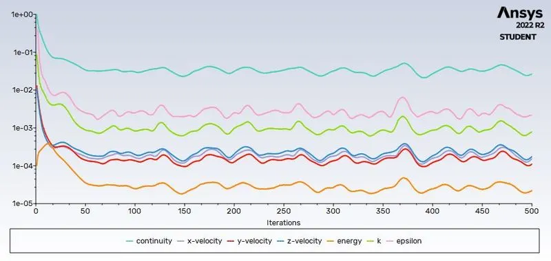
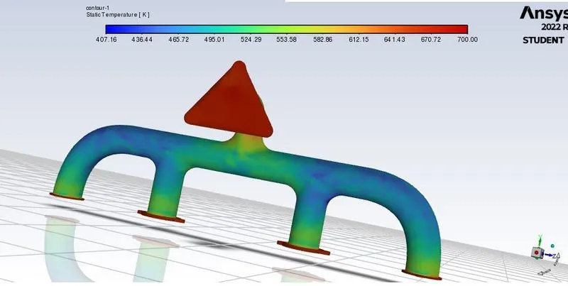
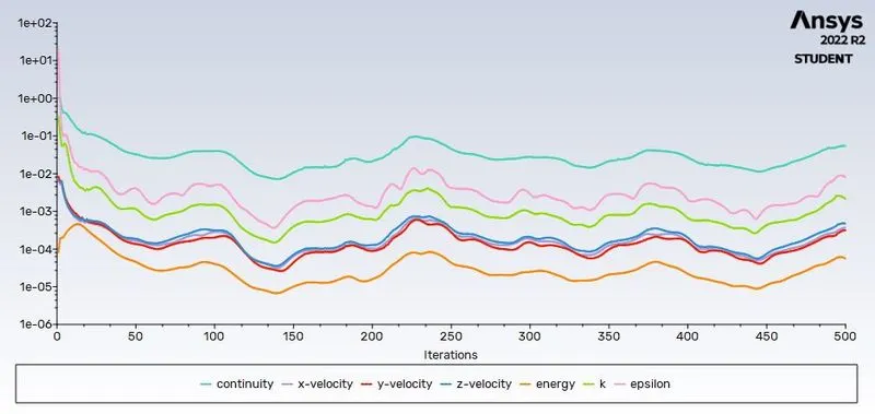
The fourth step is to initialize the solution with hybrid initialization schemes. After initialization, we create a temperature contour at the zones of the inlet, outlet, outer wall convection, and other wall regions. Give the no of iterations 500 to be performed and run the fluent solver. After convergence, check for the temperature contour zones.
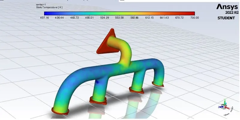
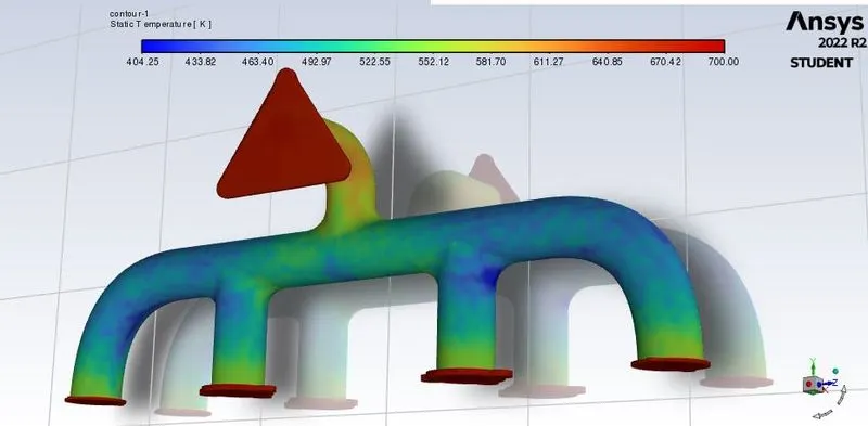
The temperature contours
The streamlines of velocity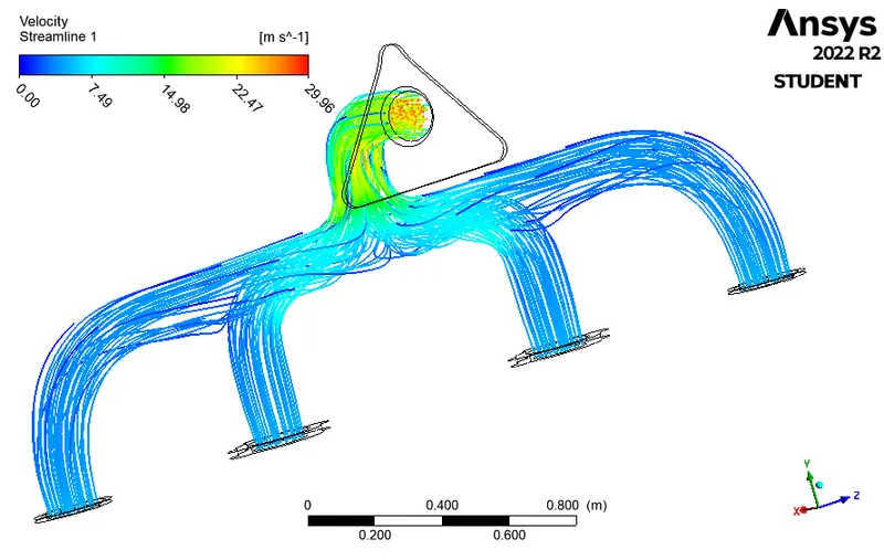
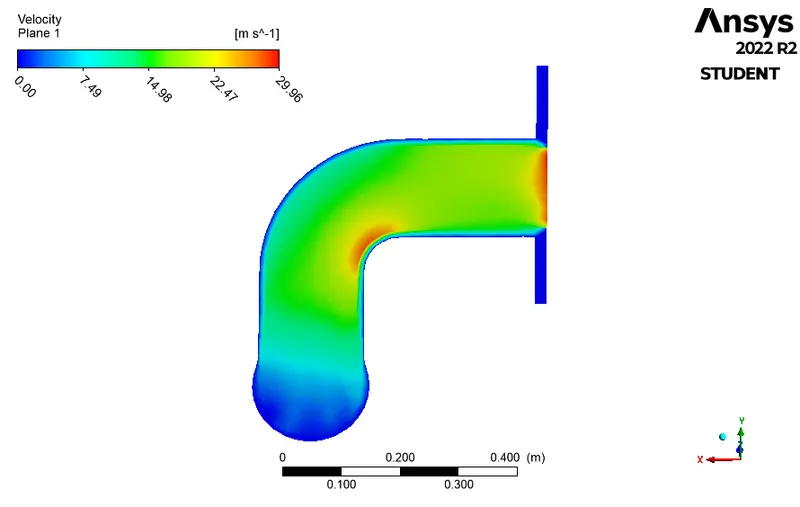
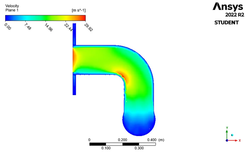
Velocity plane
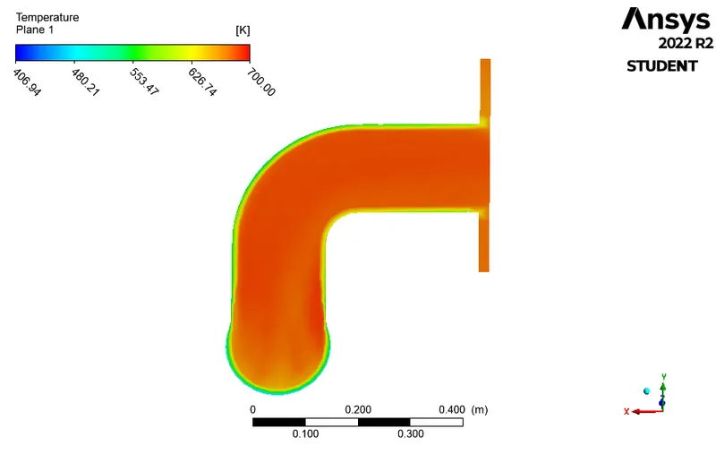
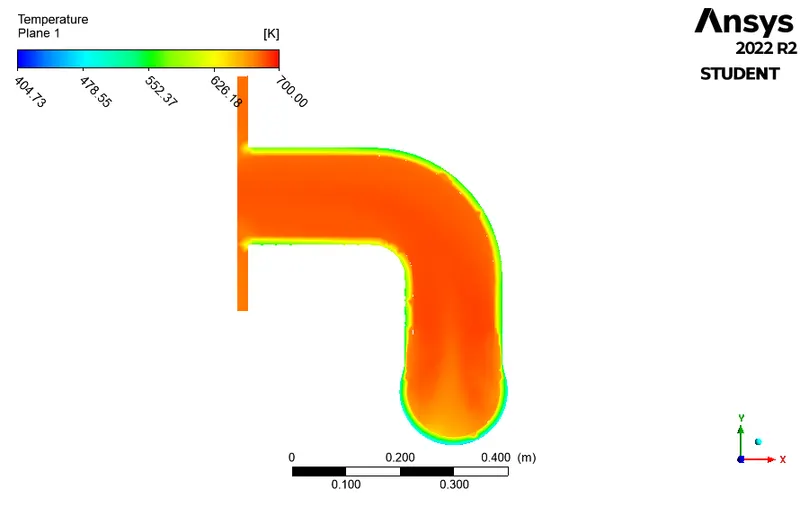
Temperature plane
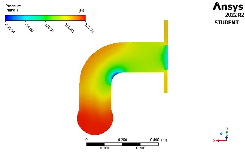
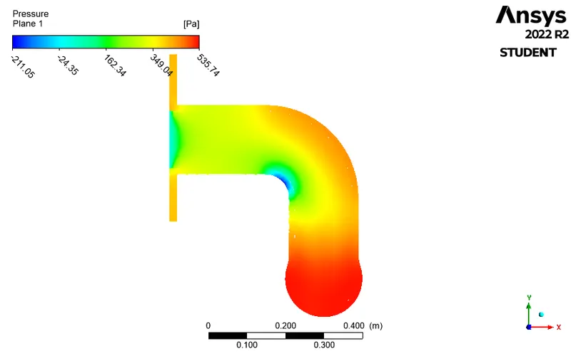
Pressure plane
Case 2
In this, the element size of the solid surface mesh is also reduced further to 15 mm size.
The Inflation layer is added to the geometry, 6 layers are added
Growth rate = 1.2
Number of inflation layers = 6
Total thickness = 5 mm
captured curvature is set to yes.
Since the value of the heat transfer coefficient takes the value of the first cell near the wall, so it can be inferred that the Y+ value will be in the viscous sub-layer which is taken to be 1
Refined mesh setup
Nodes: 148455
Elements: 443707
Meshing zone
The mesh looks like this form-
The number of elements for this mesh is 443707 and the nodes are 148455.
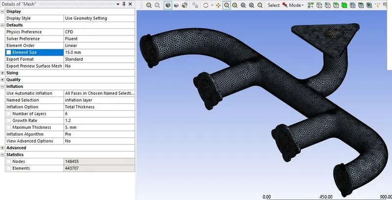
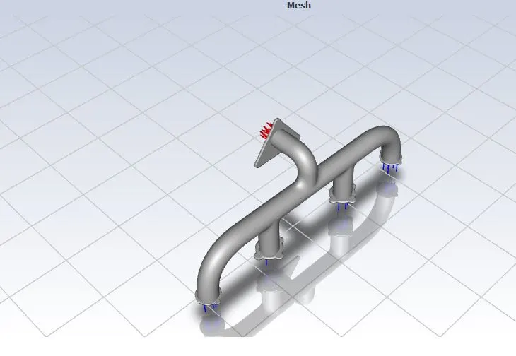
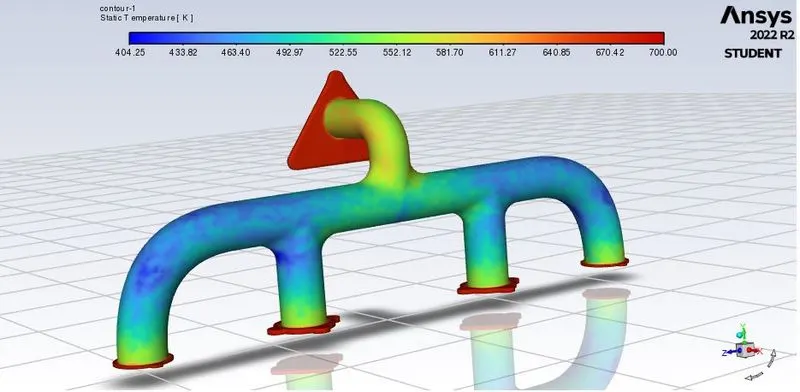
Using the same solver and the same boundary band initial conditions we get the following outcomes. Temperature contour at the zones of the inlet, outlet, outer wall convection, and other wall regions.
The plot of the residuals
Temperature plane
Velocity plane
Pressure plane
Result:
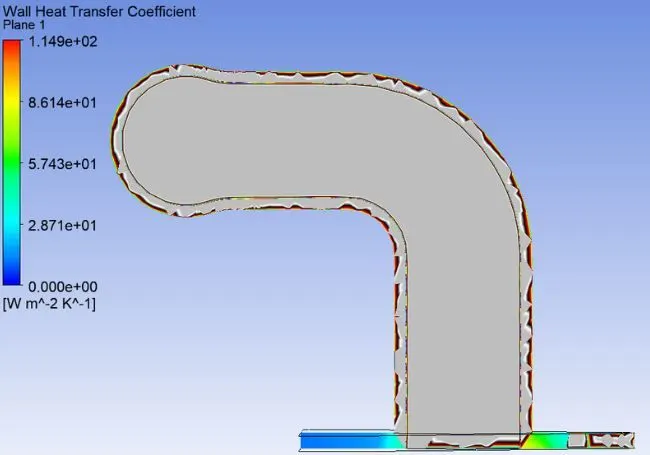
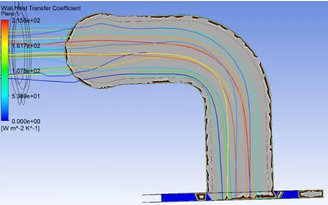
The point of the localized heat flux source is maximum at the turning point which denotes that the same point of maximum velocity will be the point of the maximum heat transfer or the max heat flux this is evident from the contour obtained.
How would you verify if the HTC predictions from the simulations are right? On what factors does the accuracy of the prediction depend on?
The typical flow conditions in automotive exhaust systems produce Re numbers in the range of 10^3 to 5*10^4. The exhaust flow often enters the region Re< 2300, especially in the exhaust manifold runners. Despite that, the flow remains turbulent, since it has flowed through a substantial restriction. The exhaust valves and the persisting, unsteady, flow pulsation effects do not favor the transition to the laminar region.
According to the Sieder Tate relation which correlates the Nu number with Re and Pr

It means Nusselt no. is the function of Reynolds no. and Prandtl no.
As the turbulent boundary layer in the vicinity of the bend at the outlet port is the thin maximum velocity of flow is observed at the bend and hence higher Reynold no.
Now, Nu = h*L/K
As the Length of the pipe and thermal conductivity are constant, the value of h will increase as Nu increases, and Nu increases as Re increases.
As per our results, the heat transfer coefficient is high for the higher value of velocity, and hence from the above discussion, we think that our results are correct.
Factors on which the prediction accuracy depends upon:
Correct choosing the value y+ which satisfies the turbulent model, by effectively capturing the velocity and temperature at the boundary wall interface.
Meshing at the junction of the solid and fluid domain. With a definite value of y+, the no of inflation layers and the growth rate determines the smooth flow of heat transfer between the two zones.
The heat transfer coefficient can be predicted by another factor called Nusselt no which is given by Nu=0.023*Re^(4/5)*Pr^n.
Factors affects the quality of prediction:
More refined mesh leads to better results.
Use inflation layers and apply proper Boundary conditions.
Proper selection of turbulence model according to y+ values.
Conclusions:
The CHT analysis on the exhaust port was simulated successfully on ANSYS-FLUENT. The conjugate heat transfer analysis is successfully performed in two cases viz baseline and refine setup. The pressure-based, coupled scheme solver is used to discretize the whole geometry.
The maximum velocity for the baseline case is found to be 29.96 m/s and for the refined case, the maximum velocity is found to be 29.92 m/s.
The velocity tends to increase from the inlet to the outlet because of mass conservation and the mixing of air. hence, the high heat transfer coefficient at the junction is due to that high velocity and also when the transfer of heat from the fluid to solid is high.
The internal flow velocity and its characteristics are affected by the Initial velocity, Pressure, the physical features of the geometry, etc. that affect the heat transfer rates, and hence CHT analysis is essential before experimental analysis for better prediction life of the designed component.
As shown in the plots, the hot exhaust gases passing through the manifold transfer some of the heat to it via convection. The amount of heat transfer can be related directly to the velocity of the exhaust. The temperature is lower where the flow is stagnating or is moving at the inlet velocity. As the velocity increases, so does the Reynolds number and hence the amount of heat transferred.
The best method to predict the accuracy of the result is by comparing the nusselt numbers from experiments and numerical results. The other method to verify is by comparing the results from published experimental results.
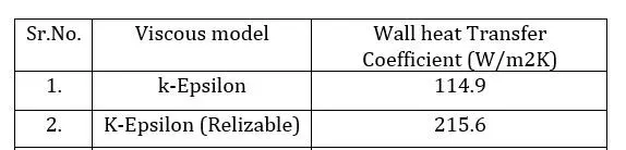
Conjugate heat analysis can accurately predict heat transfer by simultaneously solving all the relevant solid and fluid field heat transfer processes like free and forced convection in gases, in IC engine analysis, conduction through, etc. In this study, CHT analysis has been done to find out the temperature rise manifold because of hot air passing through it and we predicted the heat transfer coefficient as well. Velocity contours were created to get insights into the fluid path and maximum velocity area. It can be seen from the graph that the heat transfer coefficient is related to the wall only. Simulation is conducted for two different meshes distinguished in size. The simulation can be performed for a wider range of base mesh size values.
The grid independence test was also observed during mesh refinement. The value of the heat transfer coefficient for the first and second mesh refinement is close to each other. We must limit ourselves to the second refinement only to save the computational time and cost of the project.
The value of the heat transfer coefficient is located in the cell adjacent to the wall, allowing us to choose the value of `Y+=1` (viscous sublayer). The presence of the boundary layer is quite visible near the inlet of the pipe where the viscous force makes the velocity near the wall to be zero causing a no-slip condition to occur. The velocity at the outlet is higher than the velocity at the inlet can be attributed to the presence of four inlets and one outlet.
The values predicted by the baseline mesh and the refined mesh were close to each other this can be attributed to the fact that the boundary keeps on growing and declining from the inlet to the outlet owing to changes in velocity, thus the value is predominant at the outlet section of the exhaust port.