Week 4 - CHT Analysis on Exhaust port

Aim:

• To conduct CHT analysis on exhaust port in ANSYS Fluent.

Objective:

• A brief description of why and where a CHT analysis is used.
• A simulation of both fluid flow and also heat transfer to the solid i.e., CHT Analysis on an Exhaust port
• To calculate the wall heat transfer coefficient on the internal solid surface & show the velocity & temperature contours in appropriate areas and verifies the HTC predictions from the simulations.

EXPLANATION

Conjugate Heat Transfer (CHT) analysis :

• By exchanging thermal energy at their interfaces and transporting it via conduction within solids and additionally via convection within fluid domains, conjugate heat transfer analysis enables the simulation of heat transfer between solid and fluid domains.
• By simultaneously resolving all pertinent solid and flow field heat transfer processes, conjugate heat transfer analysis can accurately predict heat transfer.
• The combination of heat transfer in fluids and heat transfer in solids is known as conjugate heat transfer.
• Convection typically prevails in fluids while conduction frequently does so in solids. Conjugate heat transfer is seen in a variety of circumstances, including thermal radiation, free and forced convection in gases and fluids, and conduction through solids.
• The three principal ways that heat is transferred:
• Conduction is heat transfer that happens when a stationary medium has a temperature difference.
• When there is a temperature difference between two surfaces, convection is the process by which heat is transferred between them.
• The emission of energy in the form of electromagnetic waves is known as radiation (thermal radiation). There is net heat transfer by radiation between two surfaces at different temperatures in the absence of a separating medium.

Application:

• Thermal radiation
• conduction through solids
• The simulation of heat exchangers
• General-purpose cooling and heating systems.

Advantages:

• Since wall heat transfer coefficients and their local variations on surfaces are directly calculated within the model rather than relying on simplified empirical calculations, the CHT approach has an advantage over FE thermal analyses. Therefore, the CHT approach has advantages for applications where heat transfer is either non-uniform or stimulating to estimate experimentally.

SIMULATION:

• Extract the volume by selecting all the edges and name it as a fluid body
• Select the created fluid volume and solid volume and move them to a new component
• Select the properties of the body and set topology to share

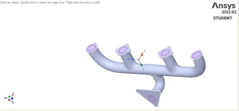
• Since it is a baseline simulation, the Ansys mesh default meshing is verified. When physics is set up, named selections are given to all the components in order to apply boundary conditions.
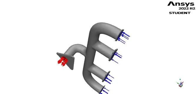
  Three options are listed: Inlets, where hot exhaust gases enter the exhaust manifold;
• outlets, where hot exhaust gases exit; and
• outer wall convection.

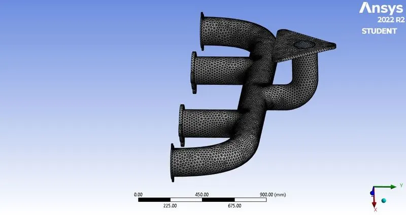
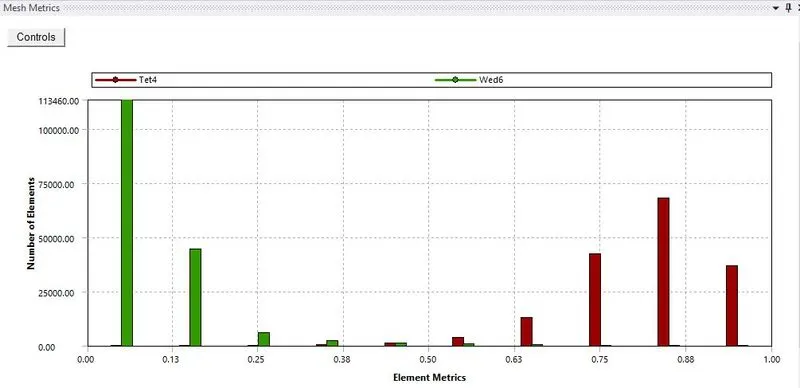
Mesh Metrics:

• The inflation layer helps us to create a body-fitted mesh. It means it creates a layer of mesh same as the geometry.

• To begin, we first chose a fluid component and gave it the name inflation layer.
  All faces in the selected named selection should be selected for automatic inflation when using the global mesh inflation option.

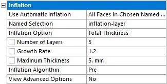
• Choose the inflation layer that we just named from the selection menu.
  Additionally, we provide the first layer thickness for the inflation option based on the y+ value and the turbulence model we employ.

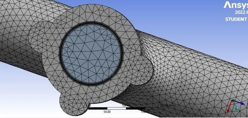
• Moving on, we choose the solver, viscous model, initial and boundary conditions, etc., in the setting up physics stage.

Boundary conditions:

Materials:

fluid - Air

Solid - Tungsten

• Inlets: For the inlets, the velocity of the fluid inflow is taken as 5 m/s and the temperature of the fluid is taken as 700 K.
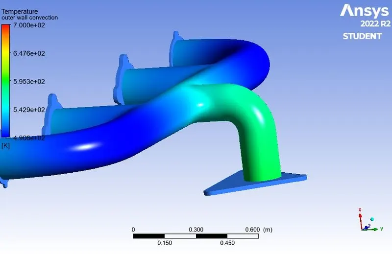
• The outer wall is considered a convection wall with a heat transfer coefficient of 20 W/m2 K.
• Outlet: Pressure boundary condition

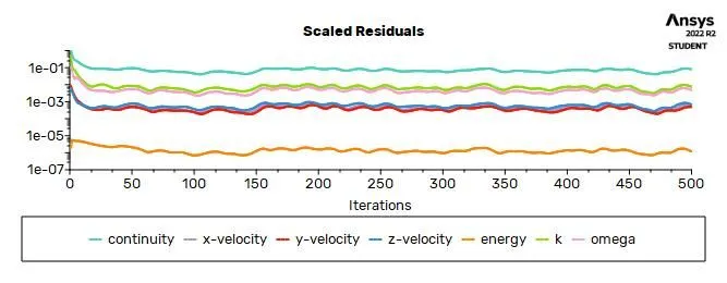
Hybrid initialization is done. The simulation is run for 500 iterations.

RESULTS:

• Residuals:

• Temperature contour:

• Velocity contour:

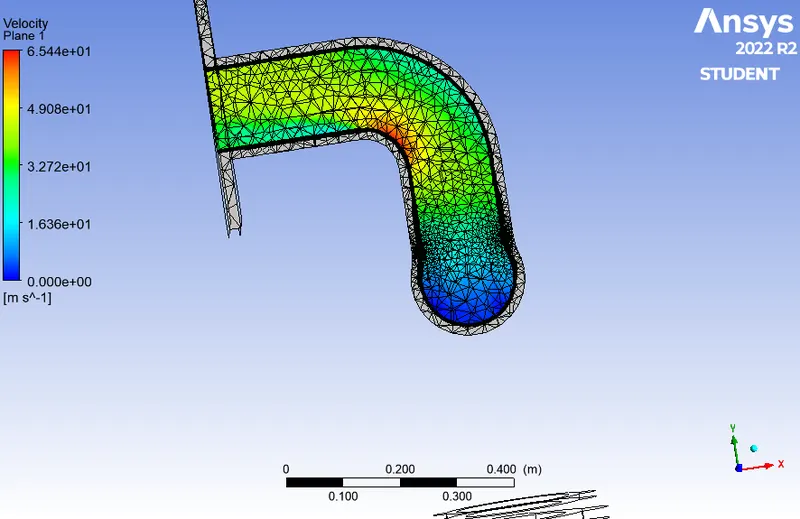
• Velocity streamline

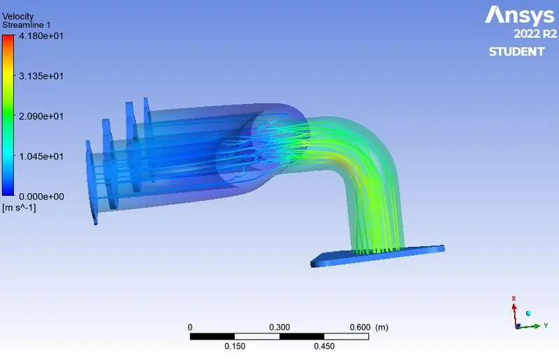
• Wall Heat Transfer Coefficient

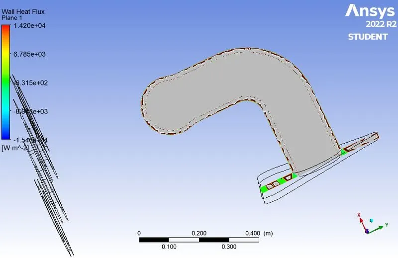
• Temperature contour

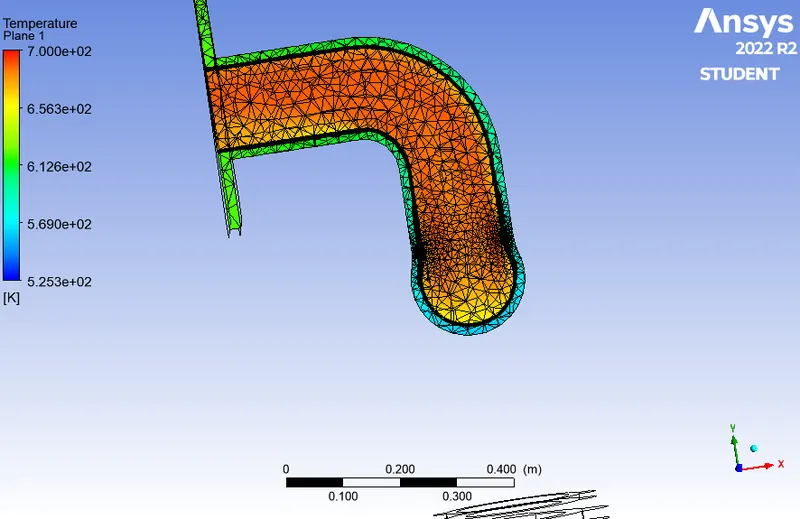
Y+ value:

• Y+ value is maintained according to the turbulence model.
• For the k-omega, SST turbulence model y+ value lies between 0.1 and 5.
• Considered y+ value = 1

Calculations:

• Freestream velocity,u = 5 m/s
• Freestream density,ρ = 1.225 kg/m³
• Dynamic viscosity,μ = 1.81 * 10 ^-5 kg/m*s
• Length,L = 0.174 m
• Y+ = 1

Reynolds Number:

Re = ρ⋅u⋅Lμρ⋅u⋅Lμ = 58881.215

Skin friction coefficient:

C_f = (0.026)/Re^1/7 = 0.005414

Wall shear stress:

ττ _wall = (C_f * ρρ * u²)/2 = 0.0829

Friction velocity:

_Ufriction = (ττ_wall / ρρ)^0.5 = 0.26015

First layer thickness:

△s = (y+ * μ)/(u_friction * ρ) = 5.695 * 10 ^-5 m = 0.06 mm

Heat Transfer Coefficient:

• The analytical value of the heat transfer coefficient is 19.4287 W/m²
• The numerical result for the HTC value is 21.4798 W/m²

Nusselt Number:

In fluid dynamics, the Nusselt number (Nu) is the ratio of the convective to conductive heat transfer at a boundary in a fluid.

Nu = hL/k

• h is the convective heat transfer coefficient,
• L is the characteristic length
• K is the thermal conductivity

Significance,

• Nusselt number is a key parameter in determining the mode of heat transfer.
• When Nu = 1, the amount of heat transfer by conduction and convection will equal.
• When Nu > 1, then the amount of heat transfer by convection is more than conduction.
• When Nu < 1, then the amount of heat transfer by conduction is more than by convection.

CONCLUSION:

• Ansys-fluent was used to simulate the CHT analysis of the exhaust port.
• The entire geometry is discretized using a pressure-based, coupled scheme solver.
• The fact that the velocity at the outlet is greater than the velocity at the inlet demonstrates mass conservation. There is one outlet and four inlets.
• Selecting the correct value for y+ and the K-omega SST turbulence model determines how accurate the heat transfer coefficient will be. When the numerical solution was compared to the HTC values predicted by CFD, the deviation was shown to be between 5% and 10%, which is acceptable by industry standards.
• The accuracy of the analytical solution, the flow characteristics, and the geometry all affect the accuracy directly. Because the boundary keeps expanding and contracting from the inlet to the outlet due to changes in velocity, the values predicted by the baseline mesh and the refined mesh were relatively close to one another.
• As a result, the value is predominate at the outlet section of the exhaust port.