Week 4 - CHT Analysis on Exhaust port

1. Give a brief description of why and where a CHT analysis is used.
2. Maintain the y+ value according to the turbulence model and justify the results.
3. Calculate the wall/surface heat transfer coefficient on the internal solid surface & show the velocity & temperature contours in appropriate areas.
4. How would you verify if the HTC predictions from the simulations are right? On what factors does the accuracy of the prediction depend on?

Solving and modeling approach

• The exhaust port was modeled into the Spaceclaim.
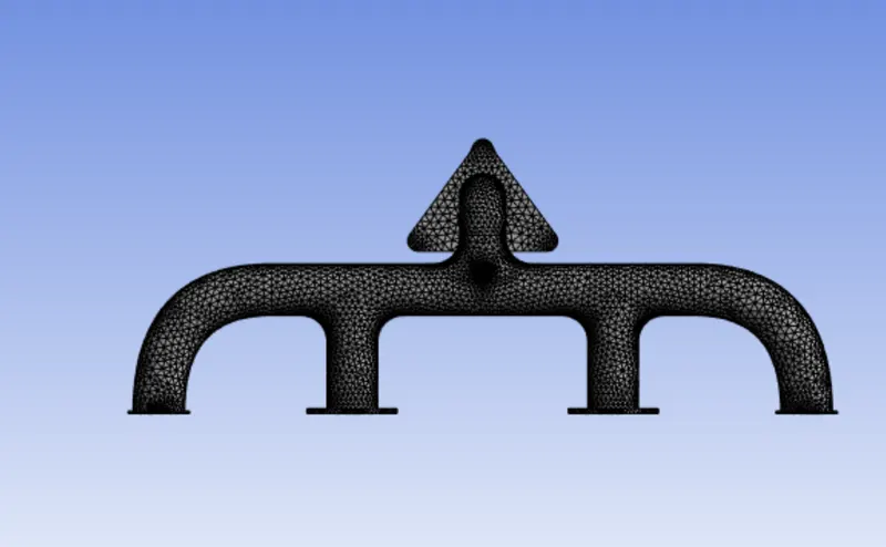
• The exhaust port is a three-dimensional model containing four inlets and one outlet. Despite having isothermal boundary conditions and a uniform flow rate at the four inlets, the model cannot be cut into two halves to save computational time because of its asymmetrical nature. Therefore the whole model is discretized and is considered for meshing.
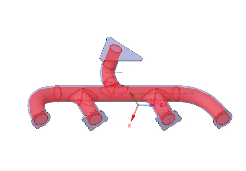
• CHT analysis requires both the solid and the liquid volume under consideration, Spaceclaim gives an option of volume extract for selecting edges for fluid volume.
• Both the solid volume and liquid volume are copied into one component.
• Share topology is created.
• Spaceclaim gives an option for share coincident topology, when share coincident topology is selected and executed, the mesh from the fluid volume and the solid volume are said to be conformal with each other which is a requirement for CHT analysis.
• The exhaust port is loaded into the meshing window and then simulated for baseline mesh and the refined mesh.
• The named selections are created ( inlet, outlet, outer wall convection)
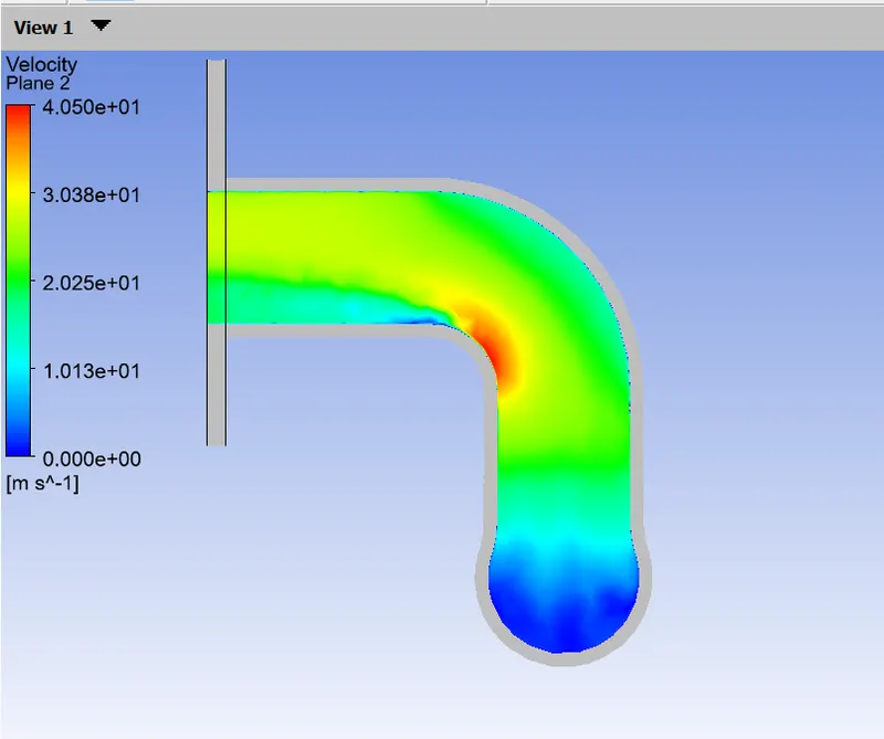
• The necessary contour images and graphs are studied to understand the behavior of temperature, velocity, and surface heat transfer coefficient at the interface.

Pre-processing and solver setting

Geometry

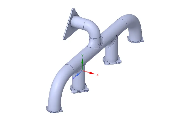
Open the Geometry with Spaceclaim and dlete the unwanted edges in the geometry for the floe analysis we internal volume go prepare volume extract select the outer edges and perform it

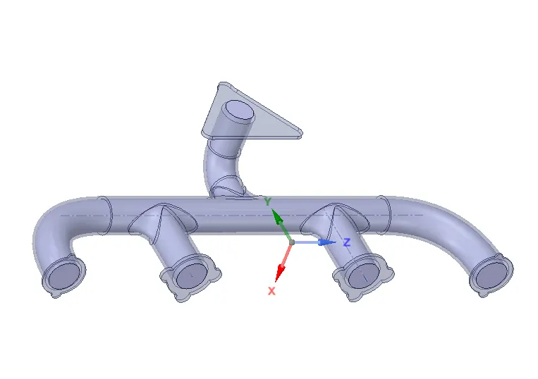
Give share topology to geometry for sharing the common node points betwen the volume and wall of the exhaust port

MESHING

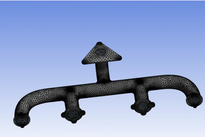
It is the process of discretizing the geometry into a small number of volumes containing nodes. Since the geometry is complex and the mesh is unstructured therefore the finite volume scheme is used as a discretization scheme.

In this case, the default element size of ANSYS-FLUENT is used 150 MM

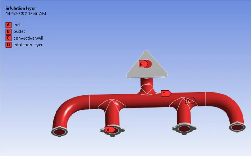
BOUNDARY CONDITION

INLET = Velocity inlet = 5 m/s

OUTLET = Pressure Outlet = 0 pa

WALL = convective wall = 20 W/m^2.K

SETUP & BOUNDARY CONDITION

Pressure based solver and steady state Condition

turn on the Energy Equation

materials

Fluid

Air

• density = 1.225 kg/ m^3
• Specific heat = 1006.43 J/kgK
• thermal conductivity = 0.0242 W/m k
• Viscosity = 1.7894e-05 Kg/m-s

Solid Aluminum for the outer shell wall

• Specific heat = 871 J/kgK
• thermal conductivity = 202.4 W/m k

Cellzone condition

• Inlet boundary condition

1. Type: Velocity inlet
2. Velocity magnitude : 5m/s
3. Temperature: 700k

• Outlet boundary condition

1. Type: Pressure outlet
2. Gauge pressure: 0pa

• Outer wall convection

1. Type: wall
2. Thermal condition: convection
3. Heat transfer coefficient: 20 W/m^2.k

SIMPLE METHOD

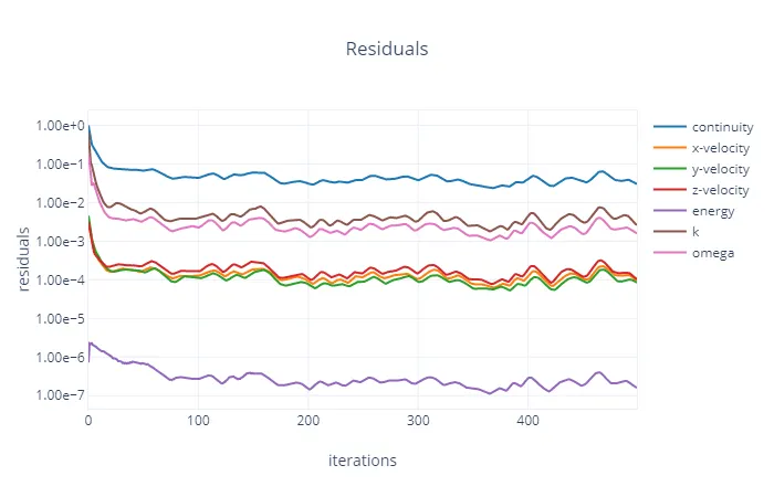
RESIDUALS

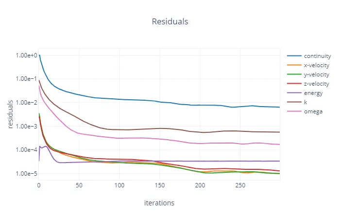
HTC

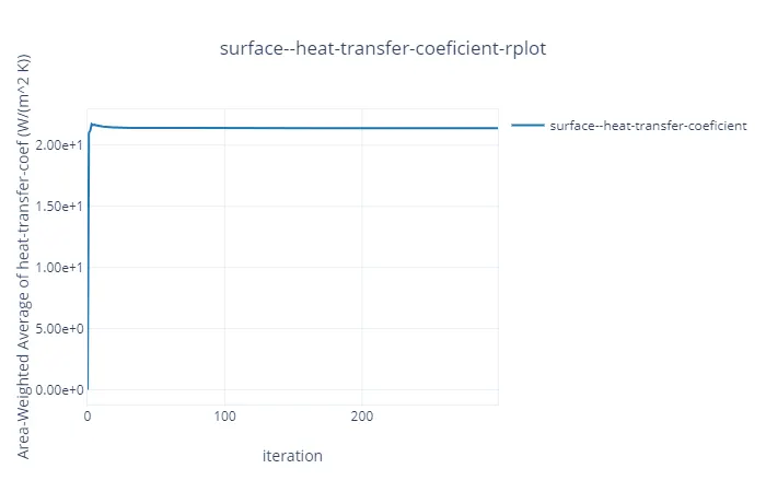
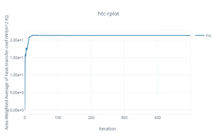
Surface heat transfer coefficient value 21.37175 W/m^2 .K

COUPLED METHOD

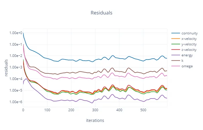
HTC

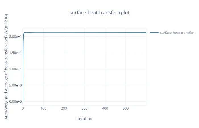
Surface heat transfer coefficient value 21.36953 W/m^2 .K

Element size cell count HTC simple HTC coupled

150mm 135980 21.37175 W/m^2 .K 21.36953 W/m^2 .K

The above table represents the value of the surface heat transfer coefficient value from the two different pressure-velocity schemes viz SIMPLE COUPLED. The values of heat transfer coefficient is exactly close for SIMPLEC and COUPLED

CHT analysis of exhaust port with finer mesh

First refinement

Element size: 100 mm

Since the value of the heat transfer coefficient takes the value of the first cell near the wall, so it can be inferred that the Y+ value will be in the viscous sub-layer which is taken to be 20.

Steps involved in calculating the first cell height.

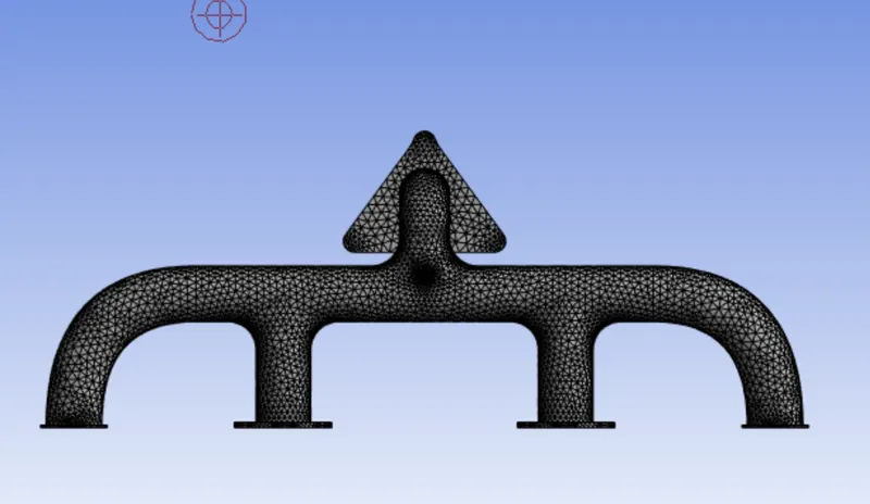
Inflation

Number of inflation layer: 5

Growth rate: 1.2

Inflation option: First layer thickness

First layer thickness: 0.5

Captured curvature is set to yes.

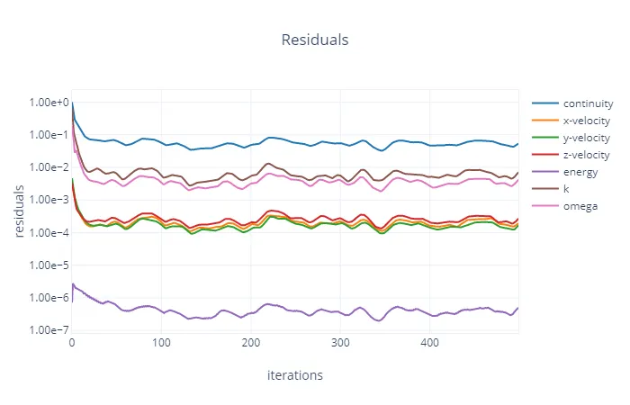
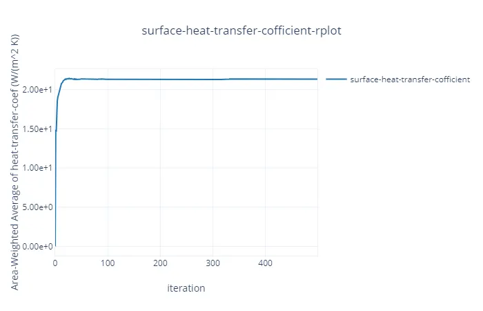
Mesh statistics and surface heat transfer coefficient

Element size	100
Number of elements	244785
Number of nodes	86109
Y+	20
First cell height	0.5
Heat transfer coefficient	21.34528 W/m^2 k

Second refinement

Element size : 50

Number of inflation layer : 5

first layer Thickness :0.5

Growth rate: 1.2

Mesh statistics and surface heat transfer coefficient

Element size	50mm
Number of elements	244843
Number of nodes	86171
Y+	20
First cell height	0.5
Heat transfer coefficient	21.33574W/m^2 k

Element size	Number of elements	Number of nodes	First cell height	Y+	Inflation layer	Surface heat transfer coefficient.(Numerical value	Surface heat transfer coefficient. (Analytical solution)
150 mm	135980		0	0	0	21.37175 W/m^2 .K	19.4287W/m^2 k
100 mm	244785	86109	0.5	20	5	21.34528W/m^2 k	19.4287W/m^2 k
90 mm	244843	86171	0.5	20	5	21.33574W/m^2 k	19.4287W/m^2 k

Result

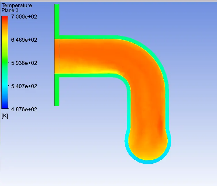
Conclusion

Conjugate heat analysis can accurately predict heat transfer by simultaneous solving all the relevant solid and fluid field heat transfer process like free and forced convection in gases, in IC engine analysis, conduction through etc. in this study CHT analysis has done to find out temperature rise manifold because of hot air passing through it and we predicted heat transfer coefficient as well. Velocity contours were crated to get insights of fluid path and maximum velocity area. It can be seen from graph that heat transfer coefficient is related to wall only. Simulation is conducted two different mesh distinguished in size. The simulation can be performed for a wider range of base mesh size values.