Week 4 - CHT Analysis on Exhaust port
AIM: To study the Conjugate Heat Transfer Analysis using the Exhaust Port.
OBJECTIVE:-
- Give a brief description of why and where a CHT analysis is used.
- Maintain the y+ value according to the turbulence model and justify the results.
- Calculate the wall/surface heat transfer coefficient on the internal solid surface & show the velocity & temperature contours in appropriate areas.
- How would you verify if the HTC predictions from the simulations are right? On what factors does the accuracy of the prediction depend?
What is Conjugate Heat Transfer Analysis : Conjugate heat transfer is a type of heat transfer analysis between solids and fluid(s). This type of heat transfer includes both convection (between fluids) and conductive (between solids) heat transfer, as well as both forced and natural convection.Typical applications of this analysis type exist as, but are not limited to, the simulation of heat exchangers, cooling of electronic equipment, and general-purpose cooling and heating systems.
What is y plus : y+ is a non dimensional measurement of distance from a wall. It is used to describe the height of the first grid element next to a wall in a CFD simulation.
Procedures :-
Geometry:
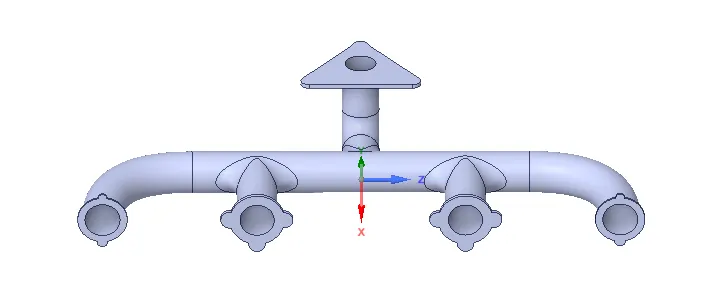
- In the space claim setup, we are setting up the CAD model geometry of the exhaust port which is already present in our system.
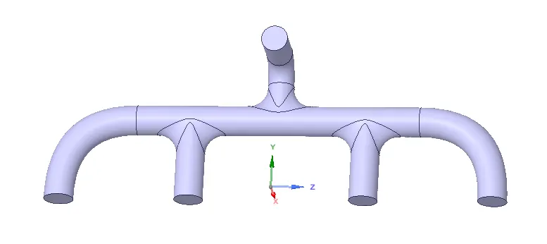
- Change the units to meters in the space claim and go to prepare Extract the volume by selecting the inner edges of the solid body.
- then go to repair remove the extra edges if any, and then go to the workbench and click on the share command and then enable the share topology.
Given geometry :
After extracting the fluid volume :
Mesh:
- We are creating the baseline mesh and then we are going to refine the mesh.
- in the mesh setup, we are using the named selection command to name the boundaries by selecting the respective face or body selection option.
- Then go to Mesh>insert>Sizing>Select solid body>assign the element size, and then in the sizing>Advance>curvature capture>yes.
- Then, Mesh>Inflation>Use Automatic inflation>All faces in chosen, and named selection>Select inflation layer, Inflation option>Total thickness, assign the number of layers, growth rate, and the maximum thickness.
- Now, generate the mesh and observing the elements and nodes in the statistics.
Number of elements = 364740
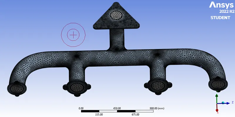
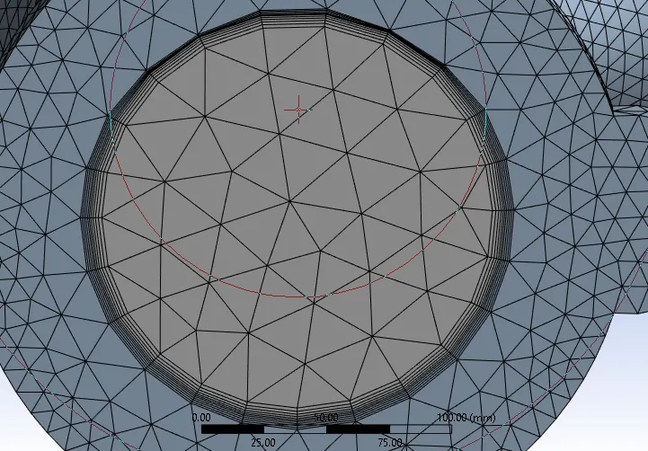
In our problem I have run 4 cases using same mesh length by changing the viscous model and inlet velocity .
Set up :
- In the setup, we are setting up the physics of the simulation.
- Setup>physics>general setting>solver>type>pressure based.
- Setup>physics>general setting>time>steady.
- physics>model>check energy.
- physics>model>viscous model>K-epsilon or K-Omega, in the baseline I have taken the K-epsilon model and for refined mesh, i have taken K-Omega, SST model.
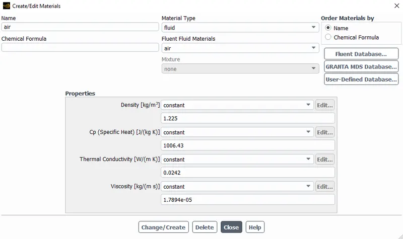
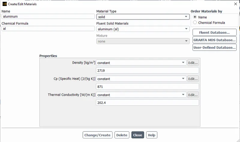
- physics> material>material type>fluid/solid.
- physics> material>fluent fluid material>air/aluminium.
- physics> material>properties> I have taken the default values here.
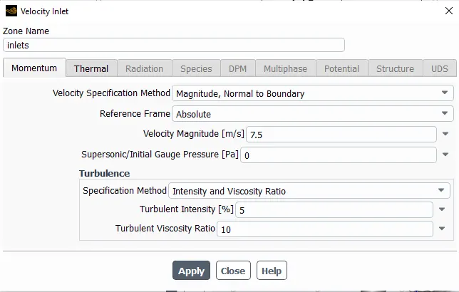
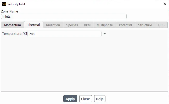
- physics>zones>boundaries>inlet> velocity as 5m/s or 7.5m/s and in thermal properties temperature as 700k and rest of all are default values.
- physics>zones>boundaries>outlet>gauge pressure as 0.
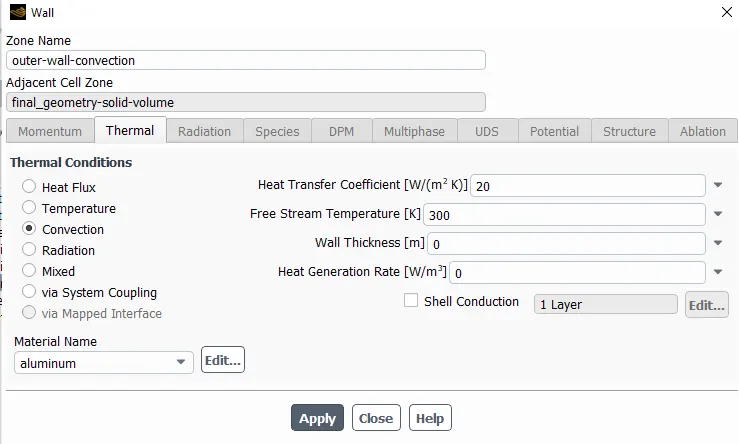
- physics>zones>boundaries>outer convection wall>thermal>convection, HTC as 20 w/m^2k, free stream temperature as 300k.
- Setup>solution>report>residuals>uncheck all the absolute convergence criteria and using the hybrid method initialize the simulation.
- and run the simulation for the required number of iterations.
SOLUTION:
In the solution, we can obtain all the simulation reports and plots.
RESULTS.
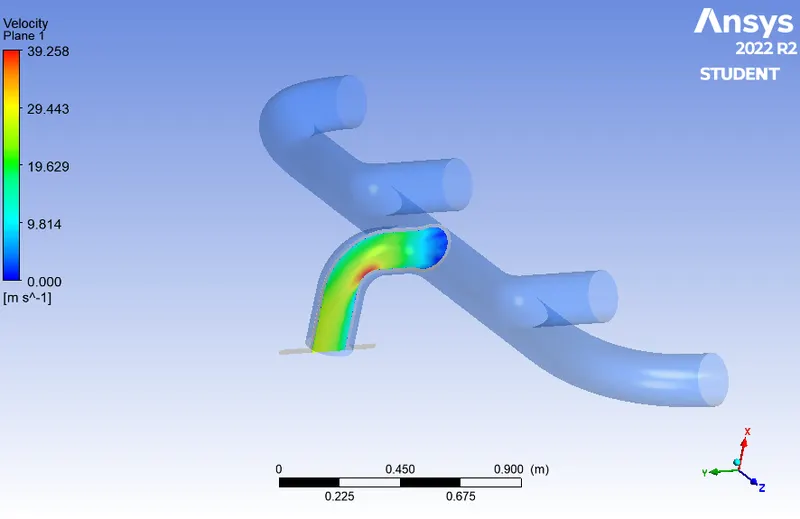
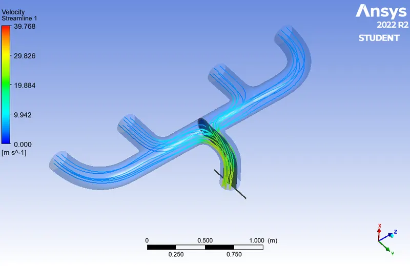
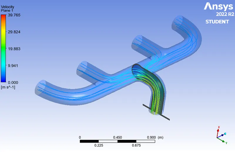
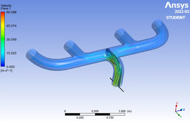
In the CFD-post we can get the velocity and temperature planes and also the streamline flow diagram for the CHT analysis.
In the below diagram we can observe the 4 inlets of the exhaust port which has blue coloured arrows and the outlet which has the red coloured arrows and the outer solid body.
Case 1 (Viscous model = K epsilon , inlet velocity = 5 m/s):
Inflation Maximum thickness: 5mm
Viscous Model: K-epsilon.
Inlet velocity: 5 m/s.
Inlet temperature: 700K.
Outlet gauge pressure: 0.
Heat transfer coefficient: 20 w/m^2-k.
Fluent material: Air.
Results:
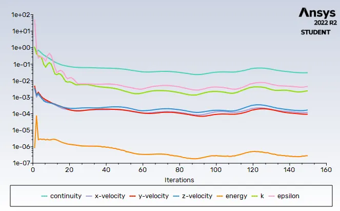
Residuals plot
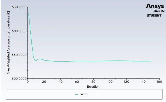
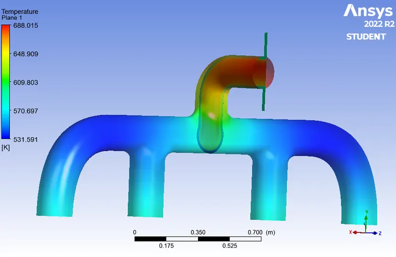
Temperature plot
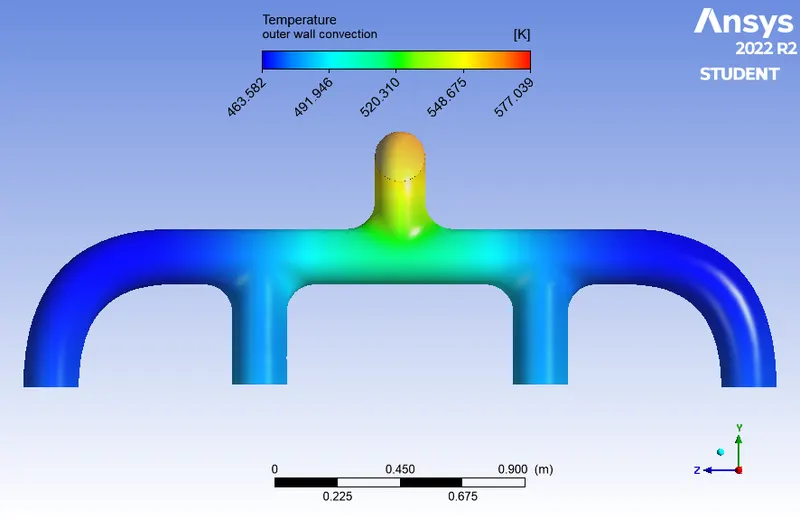
Temperature contour of outer convectuo wall
Temperature con on xy plane
Velocity contour
Velocity streamline
Case 2 (Viscous model = K epsilon , inlet velocity = 7.5 m/s):
Inflation Maximum thickness: 5mm
Viscous Model: K-epsilon.
Inlet velocity: 7.5 m/s.
Inlet temperature: 700K.
Outlet gauge pressure: 0.
Heat transfer coefficient: 20 w/m^2-k.
Fluent material: Air.
Results:
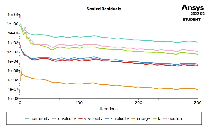
Residuals plot
Temperature plot
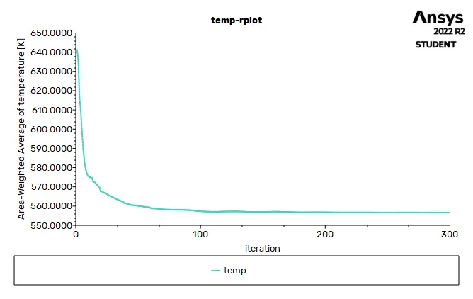
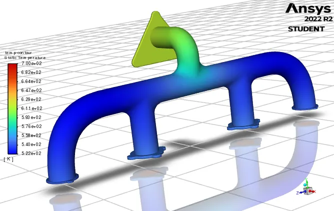
Temperature contour on convection wall
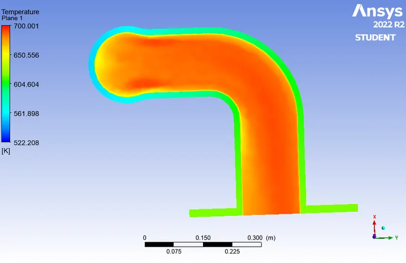
Temperature contour on xy plane
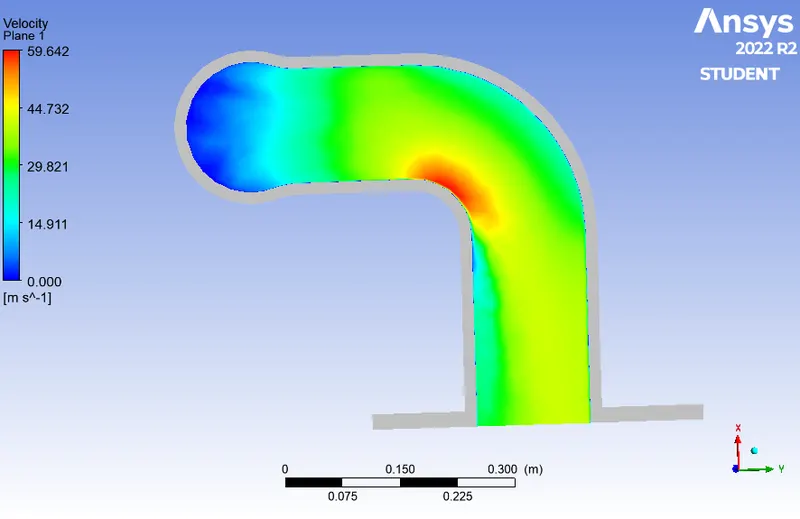
Velocity contour
Velocity streamline
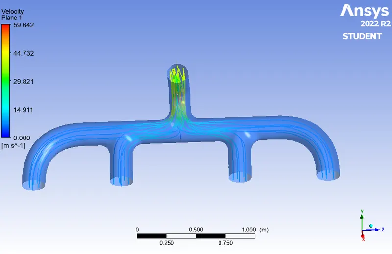
Case 3 (Viscous model = K omega SST model , inlet velocity = 5 m/s):
Inflation Maximum thickness: 5mm
Viscous Model: K-omega
Inlet velocity: 5 m/s.
Inlet temperature: 700K.
Outlet gauge pressure: 0.
Heat transfer coefficient: 20 w/m^2-k.
Fluent material: Air.
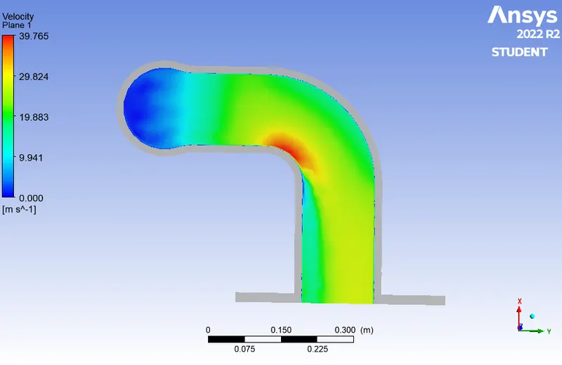
Results:
Residuals plot
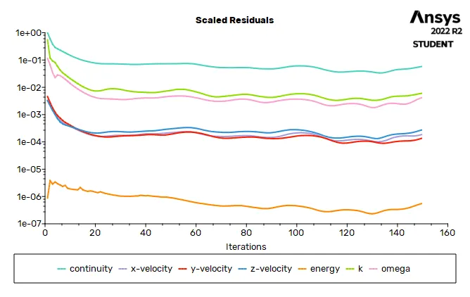
Temp plot
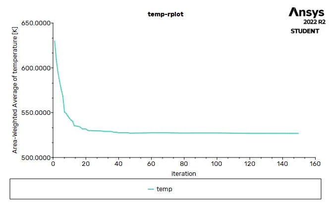
Temperature contour on convection outer wall
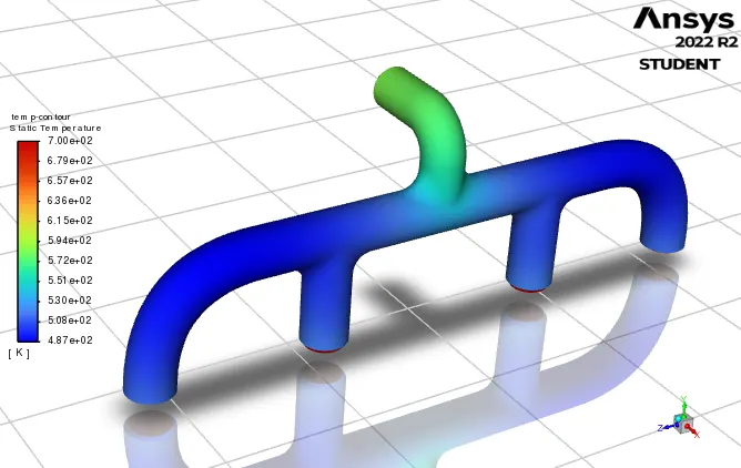
Temperarure contour on xy plane
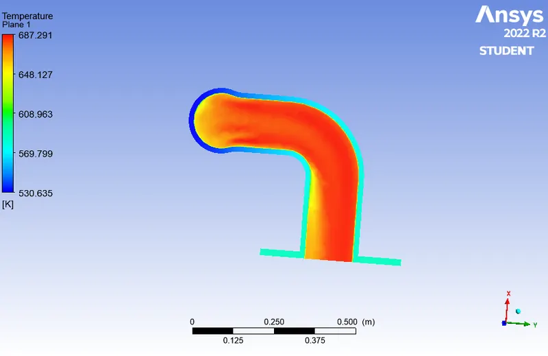
Velocity contour
Velocity streamline
Case 4 (Viscous model = K omega SST model , inlet velocity = 7.5 m/s):
Inflation Maximum thickness: 5mm
Viscous Model: K-omega
Inlet velocity: 7.5 m/s.
Inlet temperature: 700K.
Outlet gauge pressure: 0.
Heat transfer coefficient: 20 w/m^2-k.
Fluent material: Air.
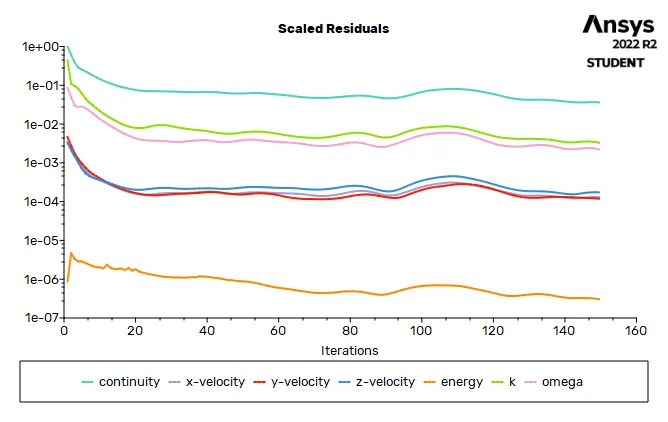
Results:
Residuals plot
Temperature plot
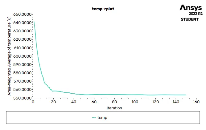
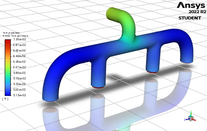
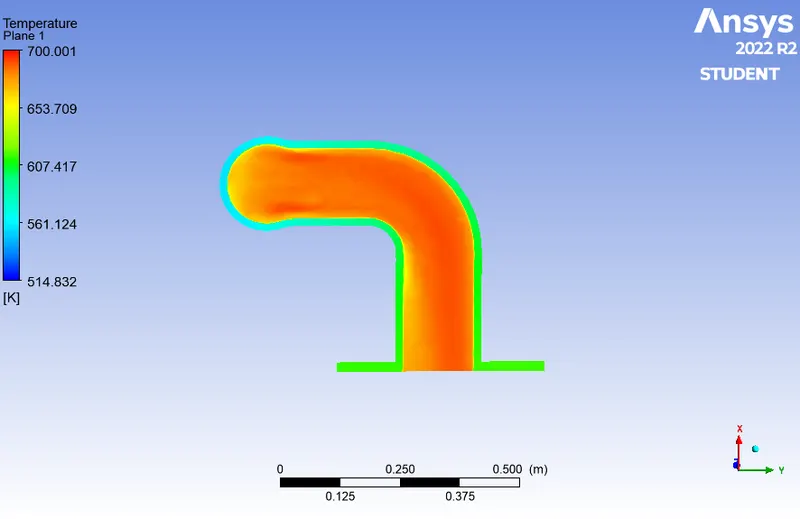
Temperature contour
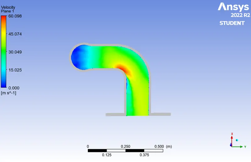
Velocity contour
'Velocity streamline
HEAT TRANSFER COEFFICIENT VERIFICATION.
Heat Transfer coefficient at boundary surface is often calculated using Nusselt number. Hence to verify the HTC obtained from the CHT analysis we first need to calculate the theoretical value of the Nusselt number.
For a turbulent flow inside a smooth pipe, Nu number is given by Dittus-Boelter equation.
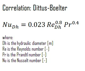
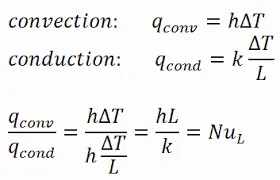
Where , Nu = Nusselt number
h = Heat transfer coefficient
k = Thermal conductivity
L = Characterstic dimension
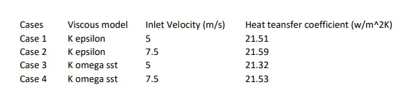
Hence, using the value of Nu from (1) we can find the value of the heat transfer coefficient, h from equation (2) and verify it with the actual results obtained from the above simulations.
Conclusion: -
1. The simulation was carried with two different turbulence model and with different velocities. From the results of residual plot we can say that Relizable K-epsilon model converge faster as compared to Standard K-omega model also later one required more iteration for stabilization. From the average temperature plot on the convection wall it was seen that Relizable K-epsilon model took lower iteration to get stabilize as compared to standard K-omega model. Whereas, from the table we can say that the percent error is lower in Standard K-omega model as compared to Relizable K-epsilon model. In the end it is beneficial to use Relizable K-epsilon model for the simulation as it was providing results faster and with great convergence ratio.
2. In all the cases we found that heat transfer coefficient increasing where value of velocity is greater which shows that increasing in turbulence cause the brownian motion to setup and cause fluid particle near to wall accelerate. Providing inflation layer is one of the best mesh input could be utilize for such simulation as we had seen in the baseline simulation it was very difficult to predict the heat transfer coefficient near the wall but after providing inflation we can get better visualization near the wall boundaries.
3.For the note on accuracy of prediction of heat transfer coefficient is greatly depend on the velocity of flow means reynolds number and nusselt number. If one calculate the arithmatic value heat transfer coefficient and provide similar to simulation then after simulation we can see it matches with calculated value.
4. Also ity is observed that with increasing of velocity or you can say Reynolds number the Hear transfer coefficient is also increasing for both of the turbulence model .
References :
https://skill-lync.com/knowledgebase/boundary-layer-y-plus-wall-functions-in-turbulent-flows-2