Week 4 - CHT Analysis on Exhaust port

Aim:

To perform a CHT analysis on exhaust port manifold.

To perform the analysis with different mesh sizes and turbulence models.

Verifying the values of heat transfer coefficient for different cases.

To Verify the HTC predictions.

THEORY :

Exhaust manifold :

The exhaust manifold is a pipe, receives the exhaust gases from the combustion Chamber and leaves it to the atmosphere. Exhaust manifolds are mounted to the cylinder head. V- Type engines have two exhaust manifolds, and an in-line engine usually has one.

This design improves breathing capacity of an engine. Exhaust manifolds are typically made of cast iron or steel, although some latest-model cars use stainless steel manifolds.Cast iron is a good material for exhaust manifolds. Exhaust gas temperature is related to the amount of load on the engine.

why and where a CHT analysis is used :

Conjugate heat transfer analysis is generally used when there is a temperature variation during heating and cooling in the material due to interaction between solid and fluid phases . The analysis of heat transfer of solid and liquid domains by exchange of thermal energy at the interfaces between them . Heat transfers in solids occur by conductions while in liquids it occurs by convection.At solid-liquid interface heat transfer takes place by convection.

CHT analysis is used in simulations of heat exchangers , engine equipments , cooling of electronic equipment and general purpose heating and cooling systems.

Application areas :

• Heat Exchangers
• Cooling of electronic equipment
• Engine equipments
• Coolers
• Heat pipes
• Heat Sink
• HVAC
• Boilers etc...

PROCEDURE :

STEP 1 : Geometry Modelling

The geometry is taken from the modelling software into the space claim

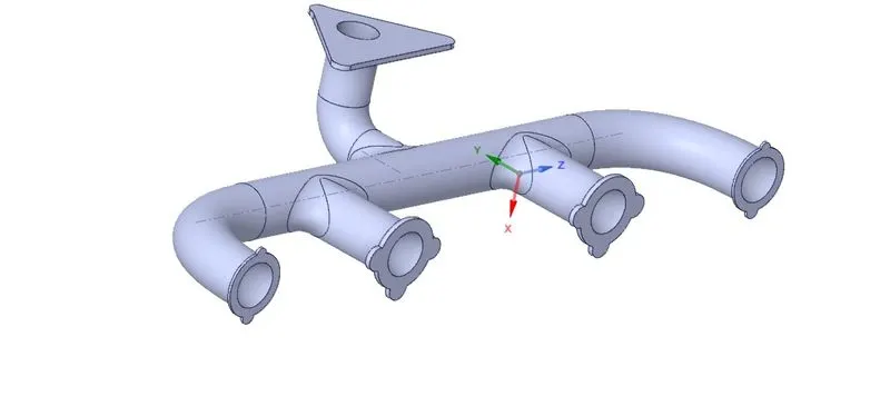
Fluid volume:

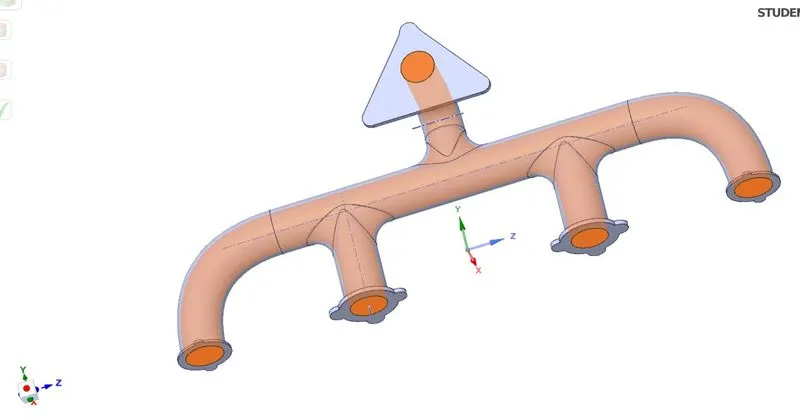
Solid volume:

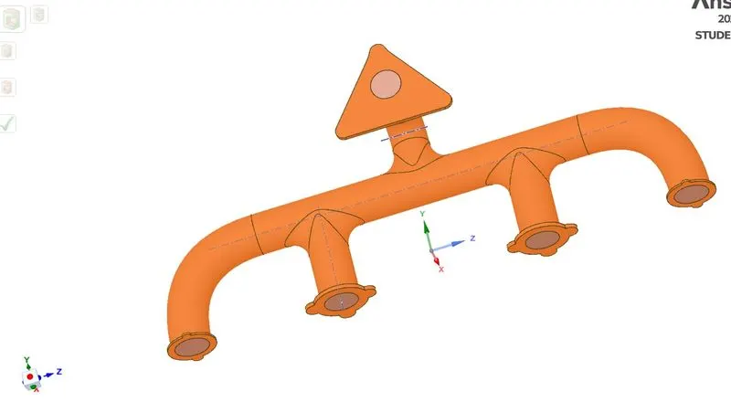
Share topology:

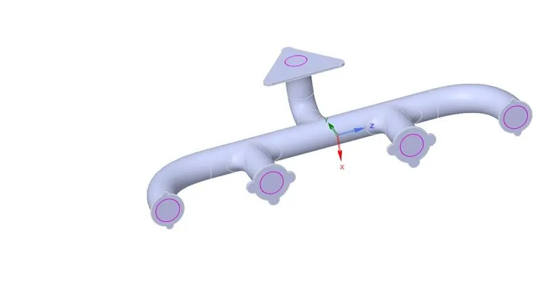
STEP 2 : MESHING

For this analysis, Base line meshinfg and Refined meshing for the different turbulence models.

Baseline mesh:

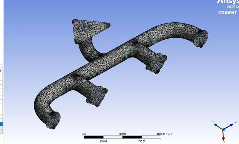
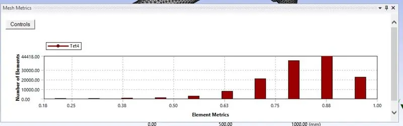
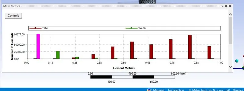
Element Quality :

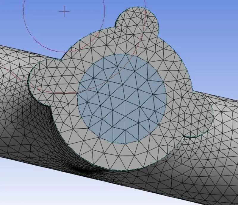
Conformal Mesh :

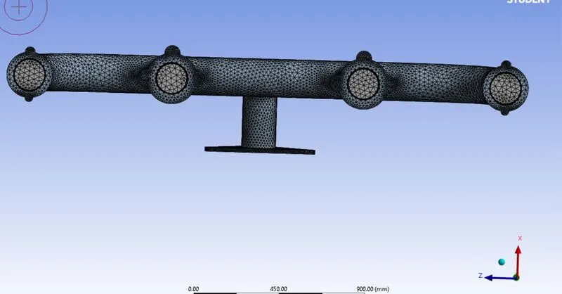
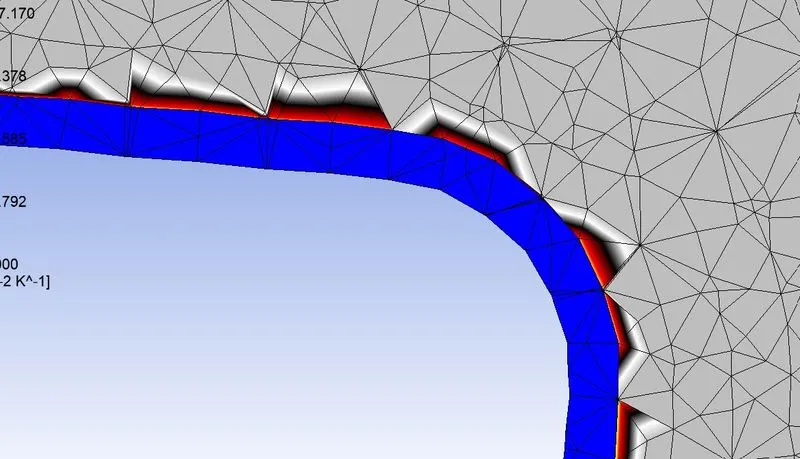
REFINED MESHING:

Element Quality :

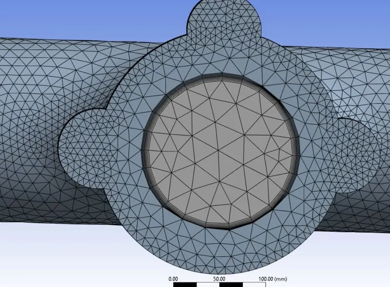
Inflation Layers :

STEP 3 : SET UP & SOLUTION

Fluent Setup

- Solver type : Pressure based

- Steady state solver

- Check the Energy equation

- Turblent Model : K-Epsilon (standard) and K-Omega (SST model)

- Fluid Material : Air

- Solid Material : Aluminum

- Intialization : hybrid

Boundary conditions

- Inlet velocity : 5 m/s

- Inlet temperature : 700 k

- Outlet pressure : 0 pa

- Outer wall Convection

*Convection with Heat transfer coefficient = 20 W/m²K

Expected Results :

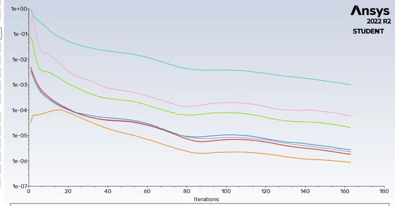
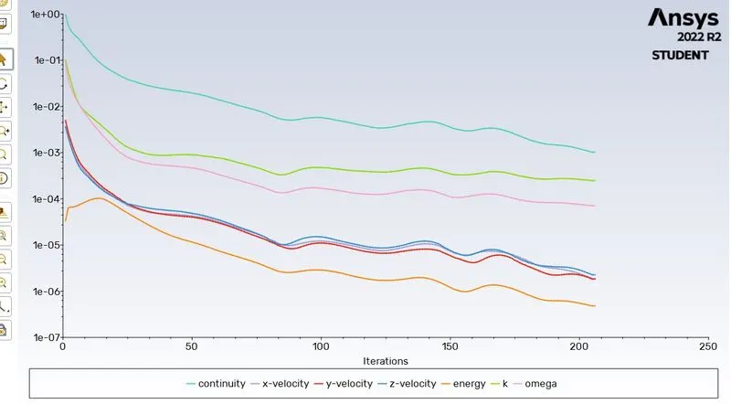
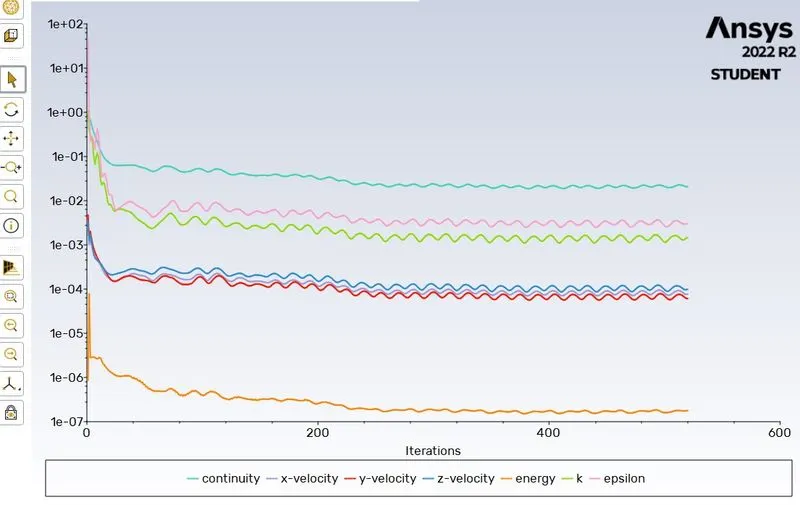
- Explaining the convergence plot getting with both the models.

- Showing the velocity, temperature, and heat transfer coefficient plots .

STEP 4 : RESULTS

BASELINE SETUP RESULTS (A)

CASE 1(A) : K-epsilon Standard Model

Residual Plot :

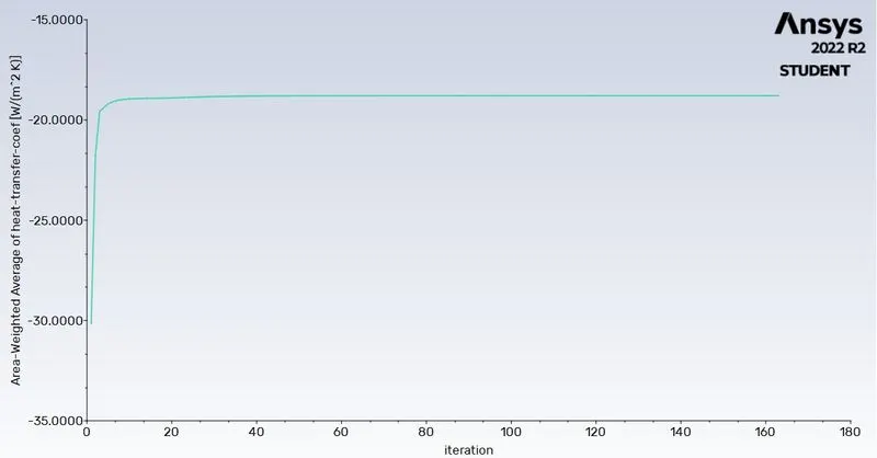
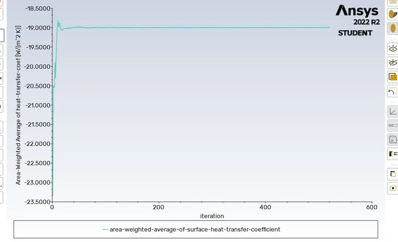
Area weighted average of surface heat transfer coefficient:

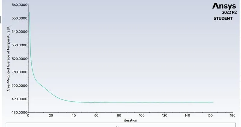
Area weighted average of outer wall temperature:

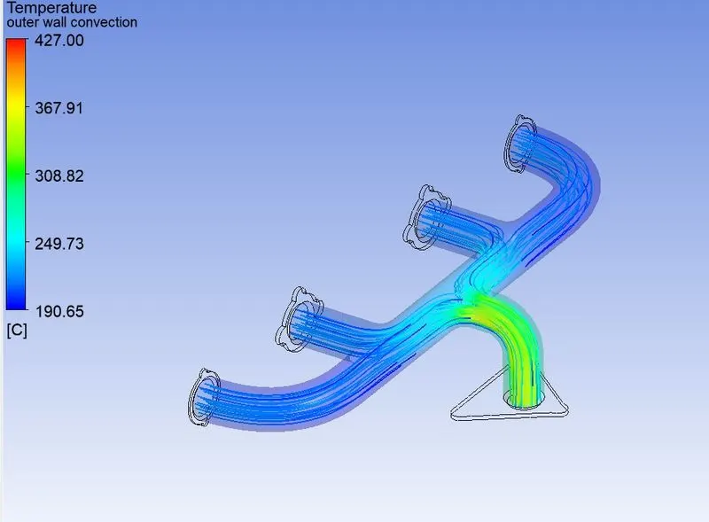
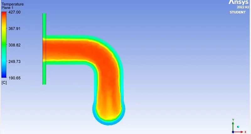
Temperature Stream-lines & contour plot :

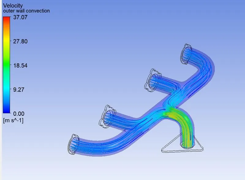
Velocity Stream lines & contour plot :

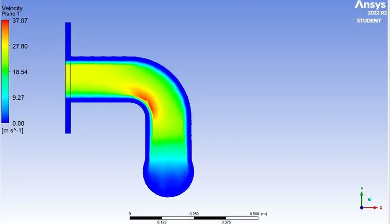
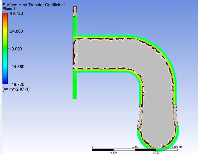
Wall Heat Transfer Coefficient :

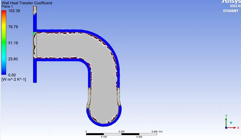
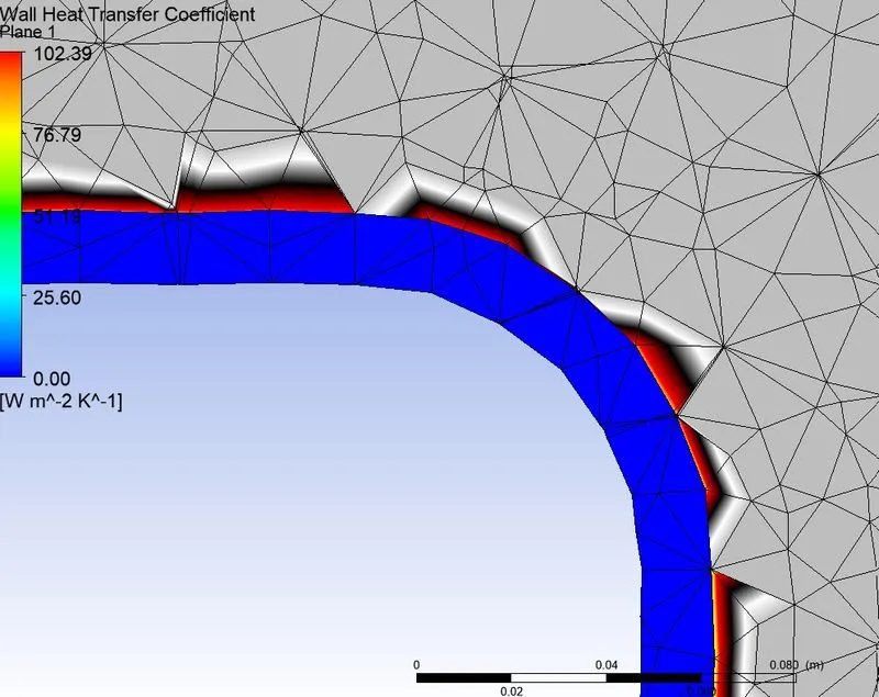
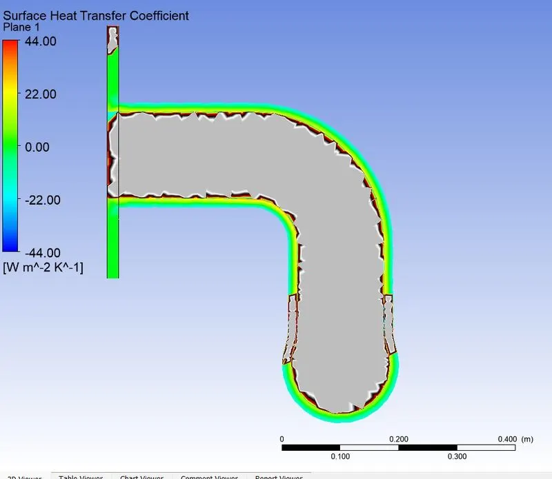
CASE 2(A) : K-Omega SST Model

Residual Plot :

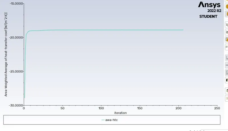
Area weighted average of surface heat transfer coefficient:

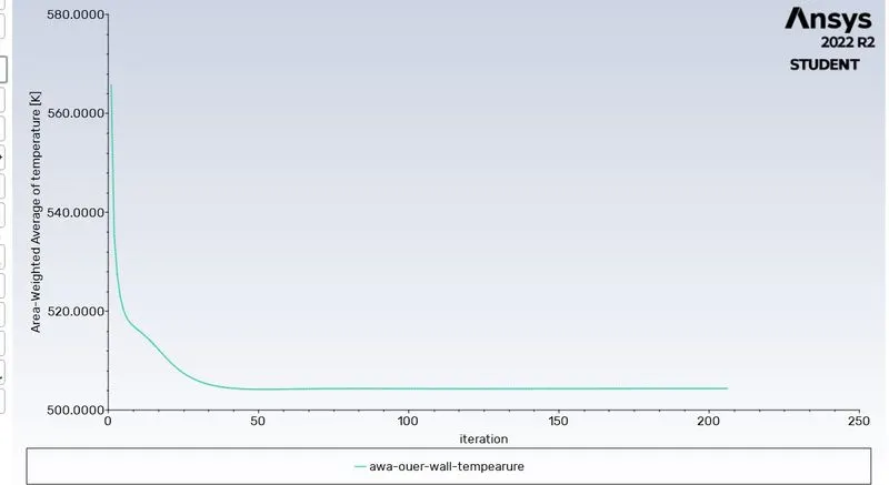
Area weighted average of outer wall temperature:

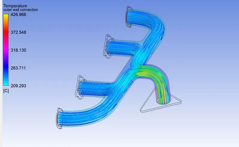
Temperature Stream-lines & contour plot :

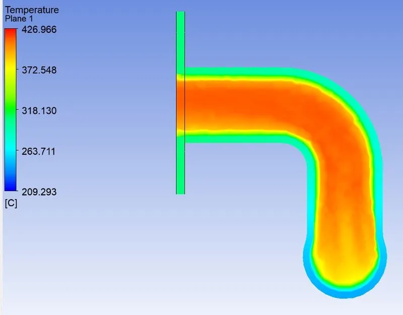
Velocity Stream lines & contour plot :

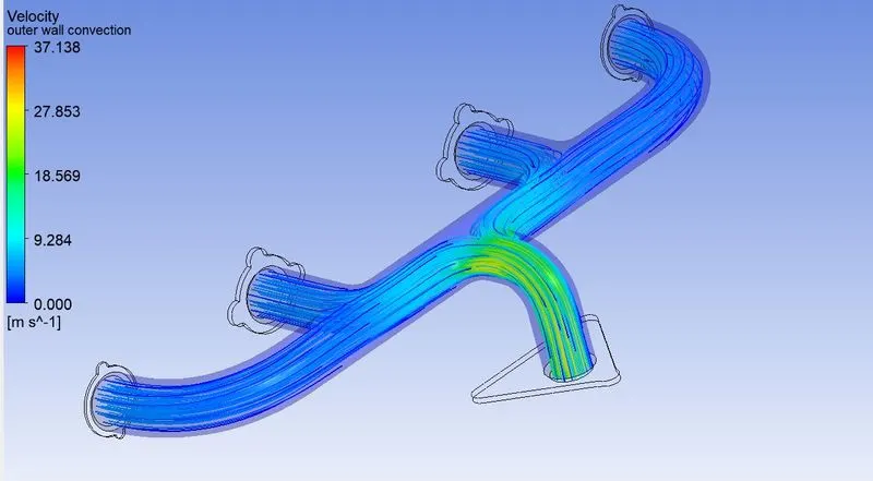
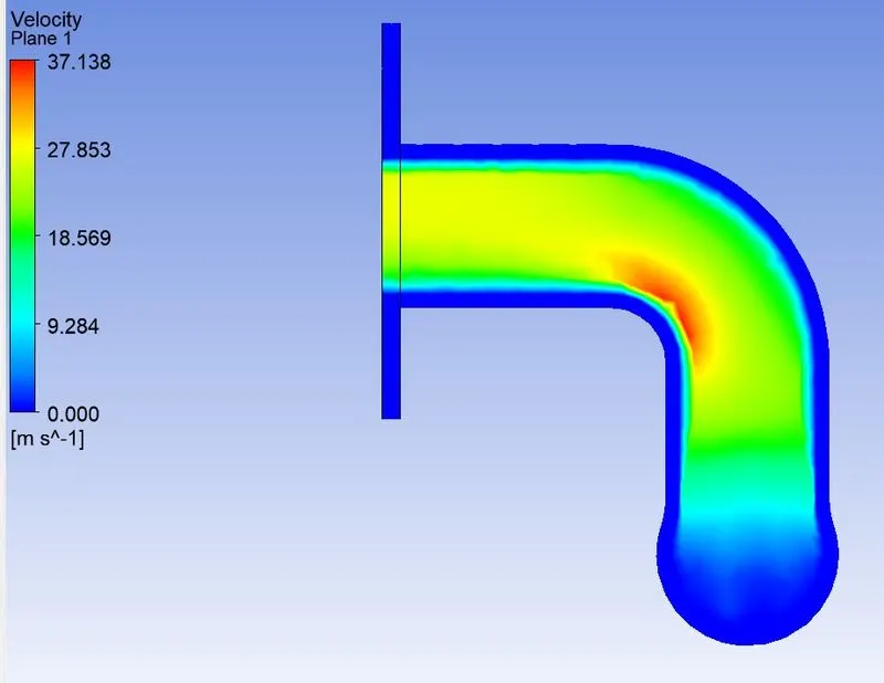
Wall Heat Transfer Coefficient :

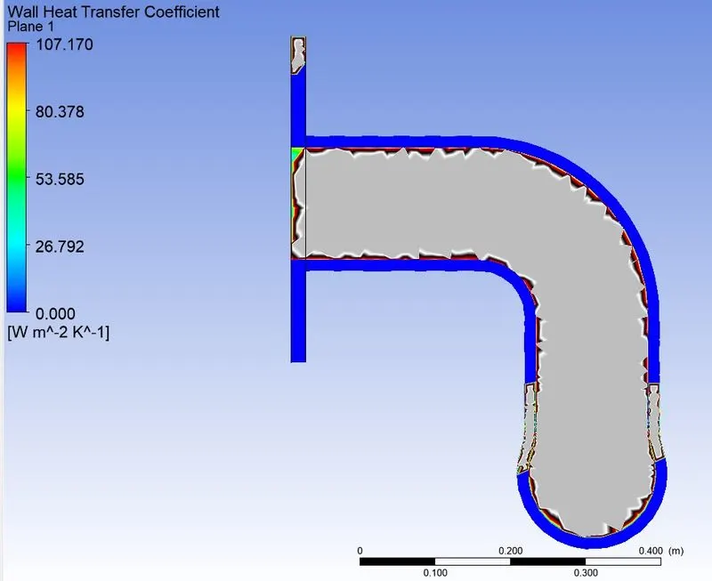
REFINED CASE RESULTS (B)

CASE 1(B) : K-epsilon Standard Model

Residual Plot :

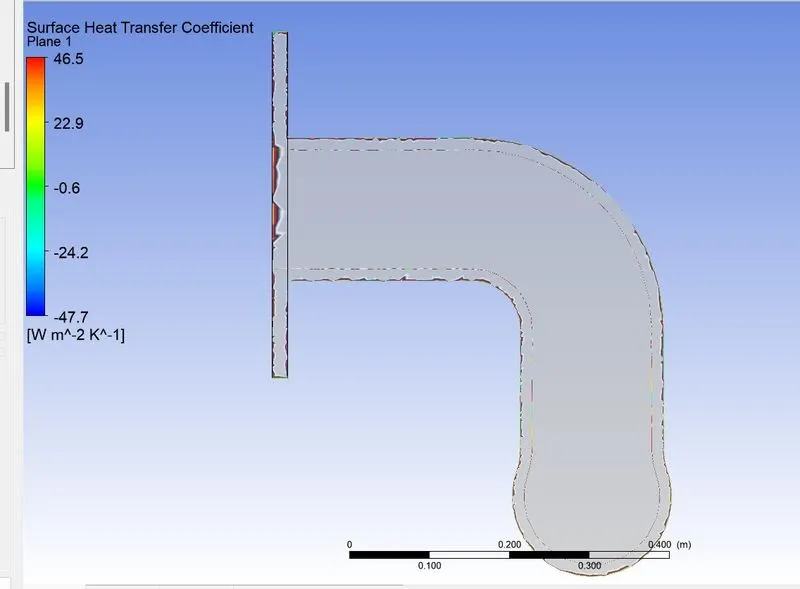
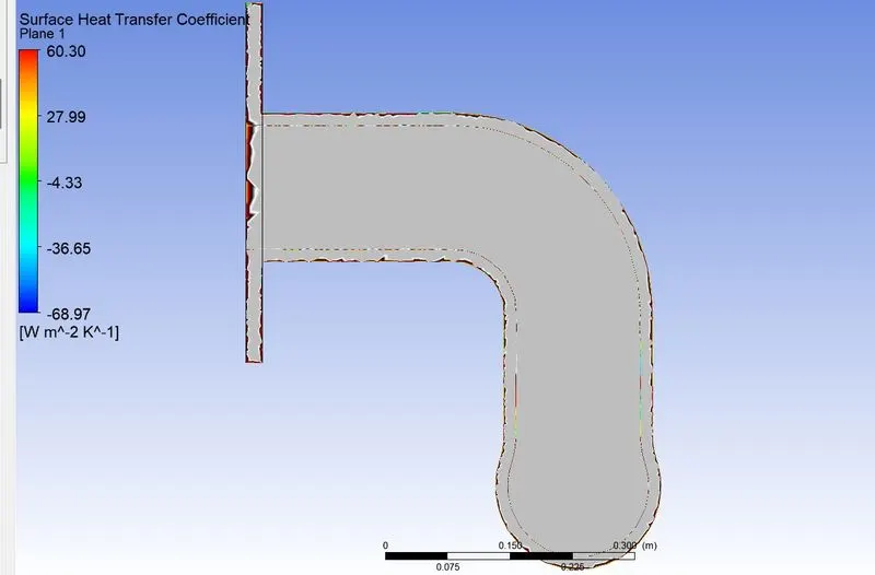
Area weighted average of surface heat transfer coefficient:

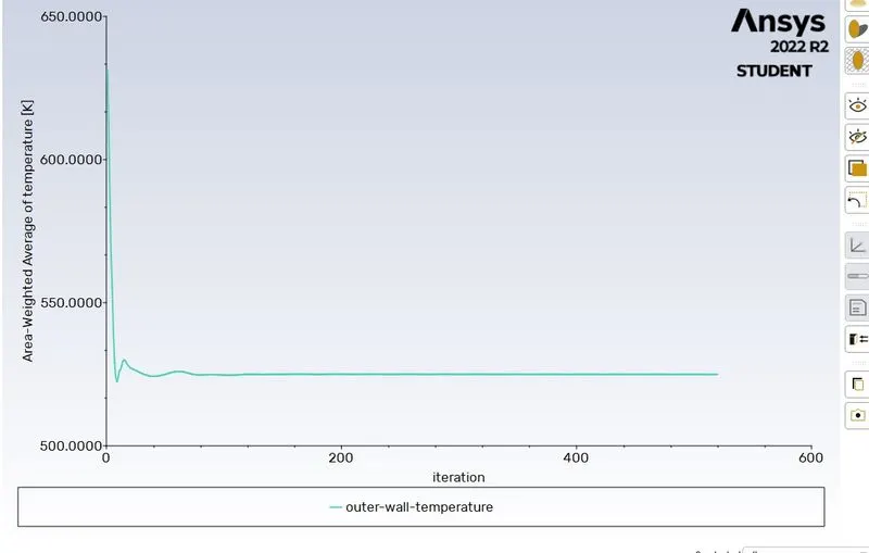
Area weighted average of outer wall temperature:

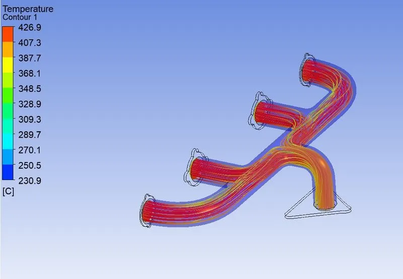
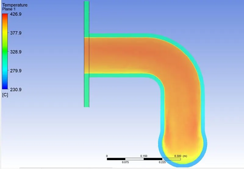
Temperature Stream-lines & contour plot :

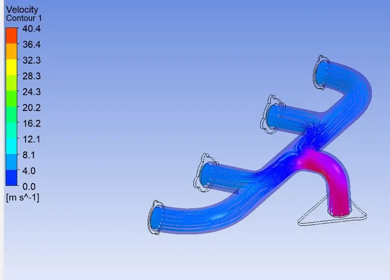
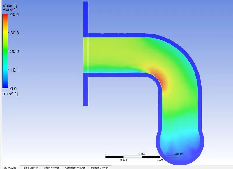
Velocity Stream-lines & contour plot :

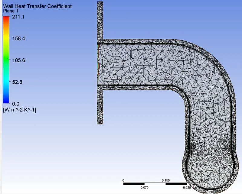
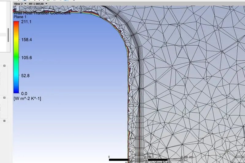
Wall Heat Transfer Coefficient :

CASE 2(B) : K-Omega SST Model

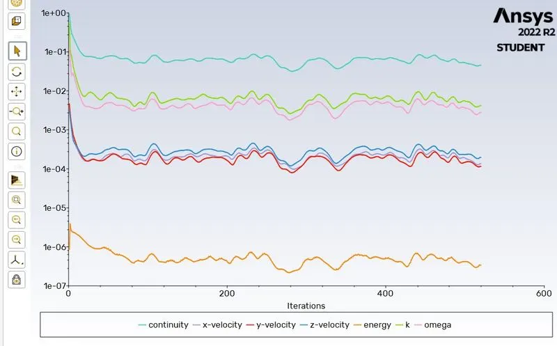
Residual Plot :

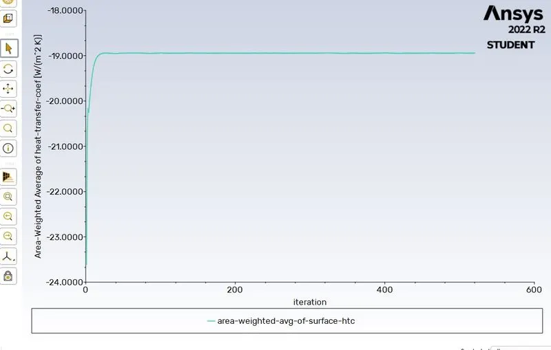
Area weighted average of surface heat transfer coefficient:

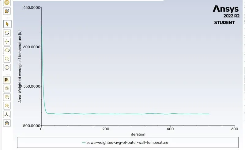
Area weighted average of outer wall temperature:

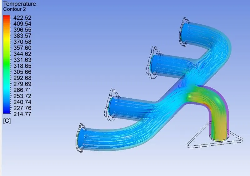
Temperature Stream-lines & contour plot:

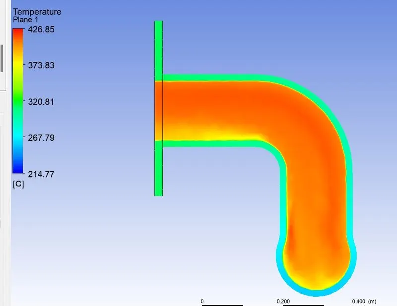
Velocity Stream-lines & contour plot :

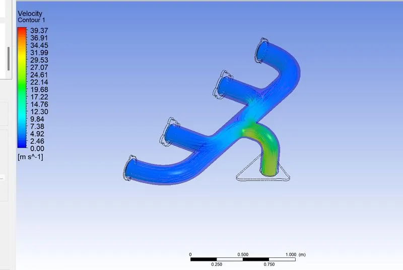
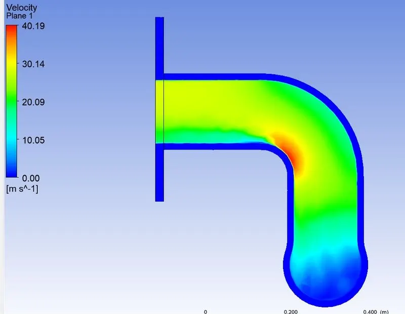
Wall Heat Transfer Coefficient :

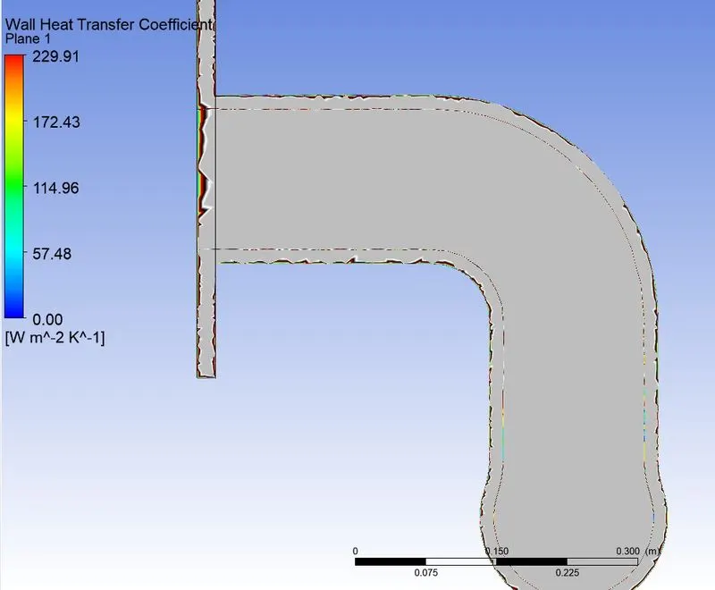
*From the above tabulated values , we conclude that K-omega SST turbulence model is more suitable for this problem.

Mesh	Model	Critical velocity(m/s)	Maximum Wall heat transfer coefficient(W/m2K)	Maximum Surface heat transfer coefficient(W/m2K)
Baseline mesh	K-epislon	37.07	102.39	44
Baseline mesh	K-epislon	37.138	107.170	49.72
Refined mesh	K-omega	40.4	211.1	46.5
Refined mesh	K-omega	40.19	229.91	60.3

Verify the HTC predictions :

Under forced convection circumstances, we can determine the heat transfer coefficient by using the Dittus-Boelter
correlation. Using the Dittus-Boelter correlation the heat transfer coefficient can be calculated in the following way using
two further dimensionless groups, the Reynolds number and the Prandtl number:

h = (k/D )*Nu

where k is the thermal conductivity of the liquid, D is the Hydraulic diameter, and Nu is the Nusselt Number which is
determined by the following equation:

Nu = 0.023Re Pr

where, n= 0.4 when fluid is being heated
n= 0.3 when fluid is being cooled

In this equation, Re is the Reynolds number which equates to:

Re = (m D )/(μ)

and Pr is the Prandtl number :

Pr = (C_P* μ)/k

For the Reynolds number, m is equal to the mass flow rate. For the Prandtl number, C_Pis equal to heat capacity, and in both
equations, μ is the viscosity of the fluid in consideration. Once we have all of these factors, we can get a decent
estimation of the heat transfer.

Also we can get the estimation from some published papers or from some experimental values.

Accuracy of HTC prediction :

Accuracy of the predictions depends on several things like,
1. Accurate geometry of model.

2. Its Mesh quality.

3. Inflation layers

4. Properties of material being used.

5. Turbulence models.

Conclusion :
1. From the above both cases output, we can say that the results are almost same but the refined mesh gives us more smoothness and accuracy.

2. Two factors influence the performance simultaneously: (a) Flow is developing along the length and the heat transfer coefficients tend to decrease along flow (b) Turbulence;

3. At the same time, turbulence is developing with tube rows at bent, which would increase heat transfer coefficients.

4. The maximum heat transfer results at bend of exit port, It is because to ensure conservation of mass at exit port velocity should more, which resuts in higher velocity and increase in velocity attain a Reynolds number that is sufficient to make flow trurbulent and higher Nusselt number at pipe bent at exit, which increses Heat transfer co-efficient at that location.