Week 4 - CHT Analysis on Exhaust port

Aim :

CHT Analysis on Exhaust port

Objectives :

1. Give a brief description of why and where a CHT analysis is used.
2. Maintain the y+ value according to the turbulence model and justify the results.
3. Calculate the wall/surface heat transfer coefficient on the internal solid surface & show the velocity & temperature contours in appropriate areas.
4. How would you verify if the HTC predictions from the simulations are right? On what factors does the accuracy of the prediction depend on?

1. Give a brief description of why and where a CHT analysis is used.

Conjugate Heat Transfer(CHT):

Conjugate heat transfer is a type of heat transfer analysis between solids and fluid(s). This type of heat transfer includes both convection (between fluids) and conductive (between solids) heat transfer, as well as both forced and natural convection. Common applications and use cases of this thermal simulation type include electronics cooling, heat exchangers, industrial machinery, some AEC cases, and more.

Numerical approaches are one of the simplest ways to realise conjugation. Iterative methods are used to set and solve the boundary conditions for the interface between a fluid and a solid. Other than by using the hit-and-miss approach, there is no way to make accurate assumptions about the values of the initial boundary condition for convergence.

Applications:

Conjugate heat transfer methods have improved as a modelling and investigational tool for natural phenomena and engineering systems in a variety of fields, including aerospace and nuclear reactors, thermal goods treatment, food processing, complex medical procedures, and ocean thermal interaction in metrology.

Through the design of heat sinks and heat exchangers for the waste treatment plant, CHT has greatly improved the cooling performance of electronic equipment in recent years. The exhaust port system is one such CHT use.

Computational Fluid Dynamics (CFD) and more specifically conjugate heat transfer (CHT) analysis can accurately predict heat transfer by simultaneous solving all the relevant solid and flow field heat transfer processes, for example: conduction through solids, free and forced convection in the gases/fluids and thermal radiation.

The CHT approach has an advantage over FE thermal analyses in that wall heat transfer coefficients and their local variations on surfaces are directly calculated within the model rather than based on simplified empirical calculations. The CHT approach therefore has benefits for those applications where heat transfer is either non-uniform or difficult to calculate empirically.

Solving the Model and approach :

1. Geometry

2. Mehing

3. Setup

4. Solving

5. Results

1. Setting up Geometry

Load the exhaust model to space claim and change the units to meters

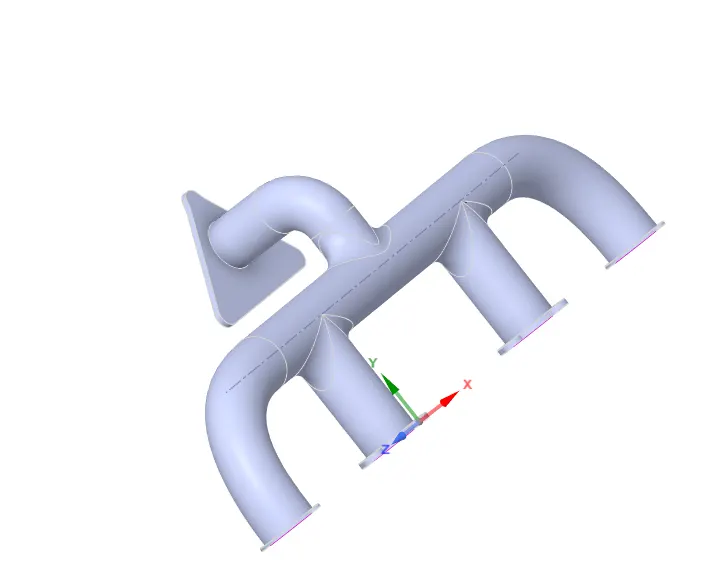
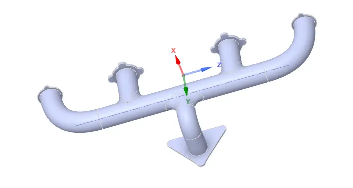
fluid volume extraction

Extraction of the fluid volume from the solid volume is what it is all about.

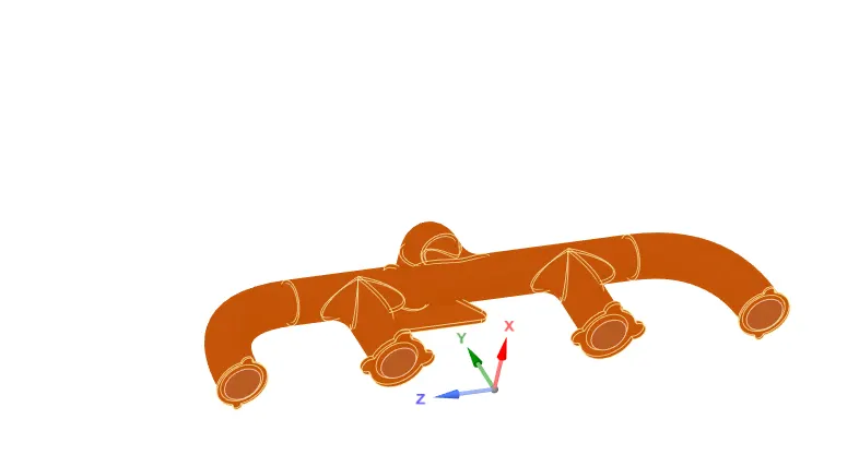
Share topology

Sharing data from fluid volume to solid volume is what it entails. It serves as a crucial criterion in CHT analysis.

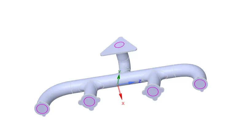
2. Meshing the Geometry :

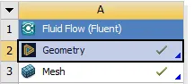
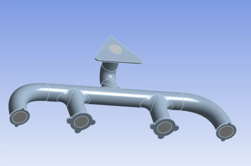
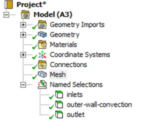
Name the section boundaries

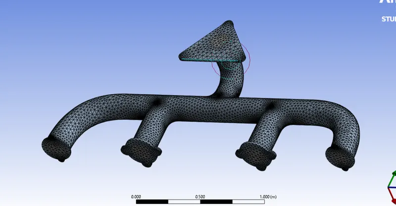
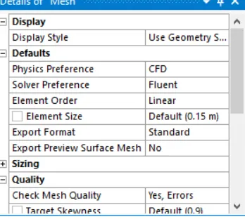
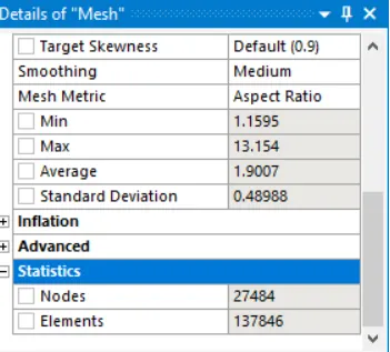
The default element size of ANSYS-FLUENT is used 0.15 m and generate the mesh

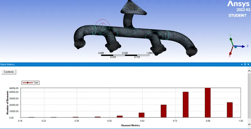
3. Geomtry setup :

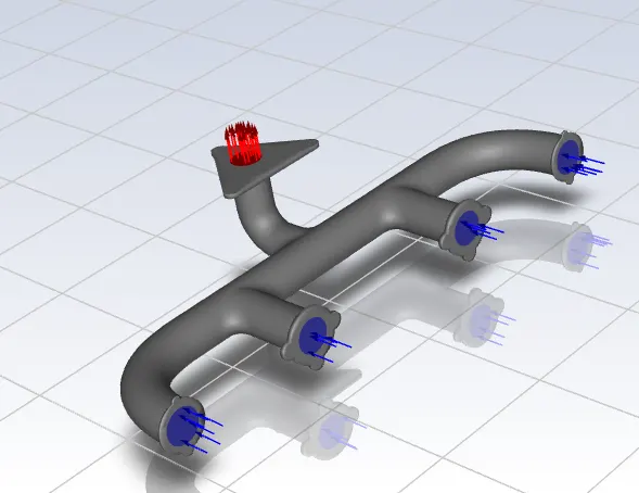
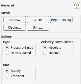
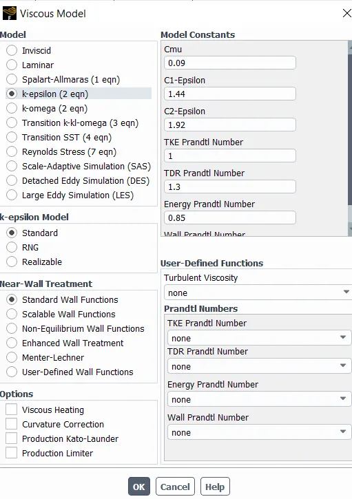
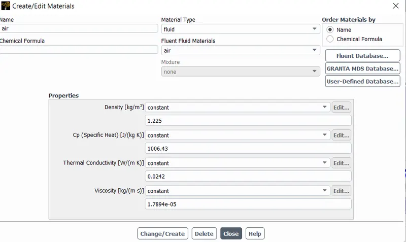
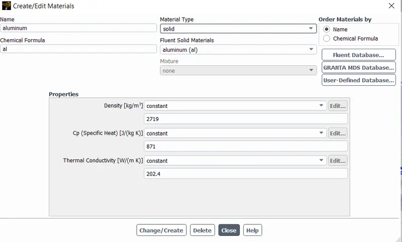
Materials :

Boundary Conditions :

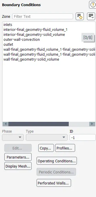
inlet

Velocity magnitude=5 m/s

temperature =700 K

outlet

pressure outlet=zero pa

outer wall

thermal=convention

Heat transfer co-eff = 20 w/m^2K

viscous model: k-omega, SST

Creatre Temperature countour :

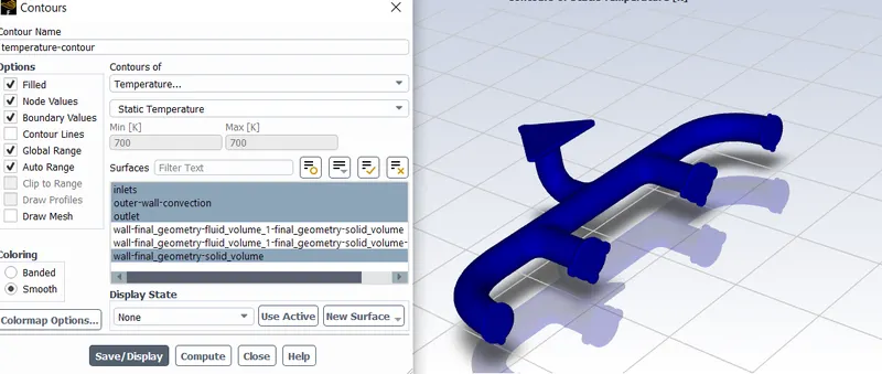
4. Solutions / outputs :

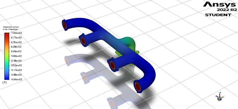
After Hybrid Intialization and run for 150 Iterations

Countour of Static Temperature

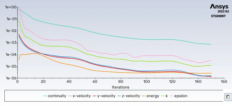
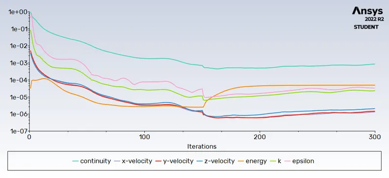
Coupled Method :

Scaled Residulals

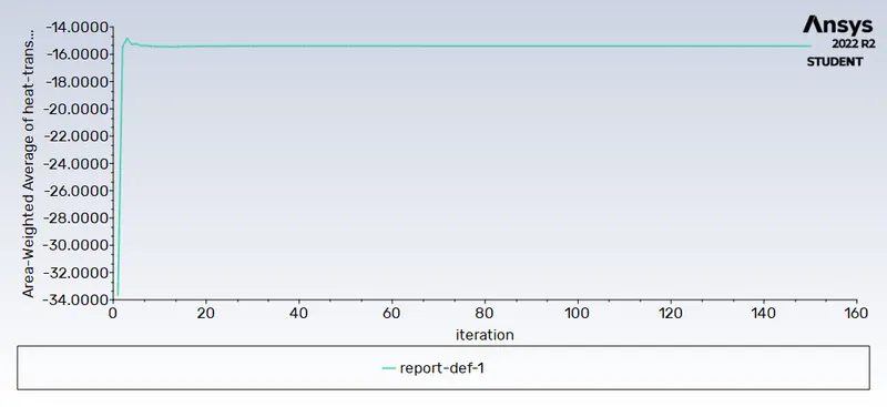
Heat Transfer Coeff :

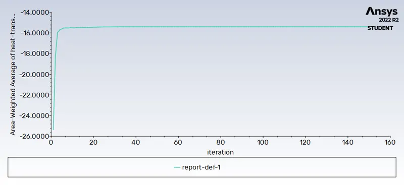
Simple Method :

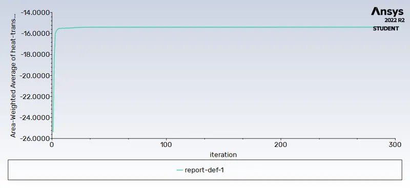
Scaled Residulas

Heat Transfer Coefficient :

Simplec Method :

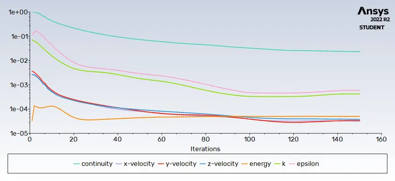
Heat Transfer Coefficient :

5. Results :

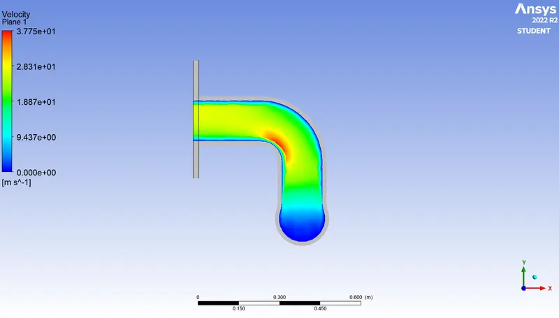
Velcoity countour :

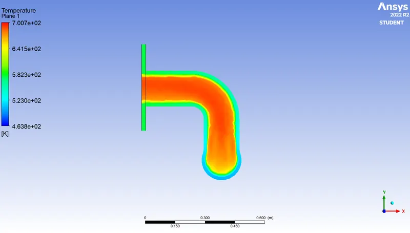
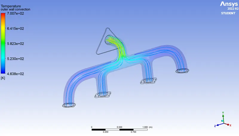
Temperature Contour :

Pressure Contour :

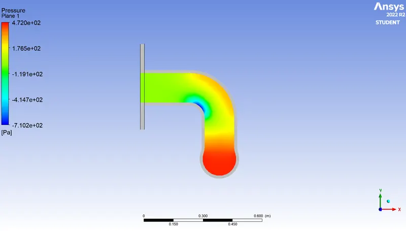
With Streamlines

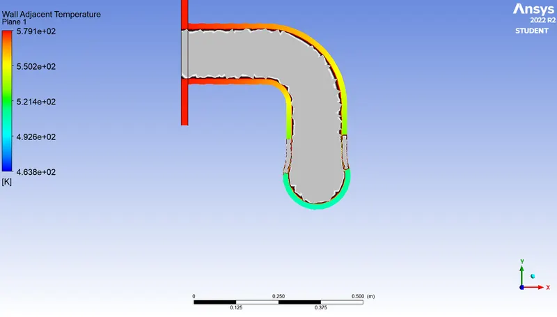
Wall Adjacent Temp :

How would you verify if the HTC predictions from the simulations are right? On what factors does the accuracy of the prediction depend on?

The typical flow conditions in automotive exhaust systems produce re in the range of 10^3 to 5*10^4. The exhaust flow often enters the region re<2300, especially in exhaust manifold runners. In spite of that, the flow remains actually turbulent since it has flowed through a substantial restriction. The exhaust valves and the persisting unsteady flow pulsation effects don’t favor the transition to the laminar region.

According to the sieder tate relation which correlates the Nu number with Re and Pr

Nu = 0.027Re^0.8Pr^1/3

It means Nusselt no. is the function of Reynolds no and Prandtl number

As the turbulent boundary layer in the bend of the outlet port is the thin maximum velocity of flow is observed at bend and hence higher Reynolds number.

Now, Nu = h*L/k

As the length of pipe and thermal conductivity is a constant value of h will increase as Nu increases and Nu increases as Re increases.

As per our result, the heat transfer coefficient is high for a higher value of velocity and hence our results are correct.

FACTORS AFFECTING THE QUALITY OF PREDICTION:

• More refined mesh leads to the better results
• Use inflation layers and apply boundary conditions
• Proper selection of turbulence model according to Y+ values.

CONCLUSION:

• Using ANSYS-FLUENT, the CHT analysis of the exhaust port was successfully simulated.
• The entire geometry is discretized using a pressure-based, coupled scheme solver.
• We can select the value of Y + = 1 (viscous sublayer) and the turbulent model k S S T because the heat transfer coefficient value is found in the cell next to the wall.

in this study, CHT analysis has done to find temperature rise at the manifold because of hot air passing through it and we predicted the heat transfer coefficient, as well as velocity contours, were created to get insight into the fluid path and maximum velocity area.

It is found that the heat transfer coefficient is more near the wall where the exhaust pipe bends.