Week 4 - CHT Analysis on Exhaust port

• Thermal interaction between the fluid and the solid region it can be either natural convection or forced convection.
• In solid region we are simulating the heat conduction. The heat conduction is basically the diffusion of heat due to direct contact.
• In fluid regions we are dealing with the convection of heat. This is the kind of transfer of thermal energy due to the movement of fluid elements.
• At the interfaces between this two region there will be a thermal coupling. Because we are considering the transfer of mass and thermal energy at the same time both in solid and fluid and also we can consider the other methods of heat transfer which is radiation.
• In CHT analysis, thermal radiation also accounts for a equal share as engineering problems does not limit to conduction and convection.
• The principle of conduction is governed by Fourier's law of heat conduction, whereas convection is influenced by Newton's law of cooling.
• In engineering applications, heat transfer problems are complex to solve due to such combination of modes of heat transfer.
• These problems are tedious to solve through conventional (analytical) means and therefore creates a need for a numerical model which can approximate the physical process.
• CHT analysis is beneficial in accurately predicting solid temperature and heat transfer capabilties in engineering devices.
• Thermal engineers in industries are responsible for controlling heat transfer capabilities for their product to ensure efficient working as per standards.

Applications of CHT :

Cooling of electronic devices - This de,Heat exchangers, HVAC (Heating Ventilation and Air Conditioning), Air-cooled and liquid-cooled engines, turbochargers, cooling of nuclear reactors, cooling towers, and many more.

CHT analysis of exhaust port

Geometry –

• We start by importing the exhaust port model into the Spaceclaim, since it’s an asymmetric model, we can’t cut the model into half in order to save computational power and hence the whole model will be messed for our analysis.
  
  
• As we are doing the CHT analysis we need both the solid volume and also the fluid volume so as to find the heat coefficient and everything else required from this analysis.
  
  
• To extract the fluid volume, we can use the volume extraction option given in spaceclaim. Then finally both the solid volume and the fluid volume are copied into a same part and the empty parts are deleted and we get the required geometry.
  
  
• Since there are two different volumes, we need to setup the share topology option so as to get a well-connected/conformal mesh between the two volumes.
  
  
• Spaceclaim gives an option for share coincident topology, when share coincident topology is selected and executed, the mesh from the fluid volume and the solid volume are said to be conformal with each other which is a requirement for CHT analysis.

Geometry :

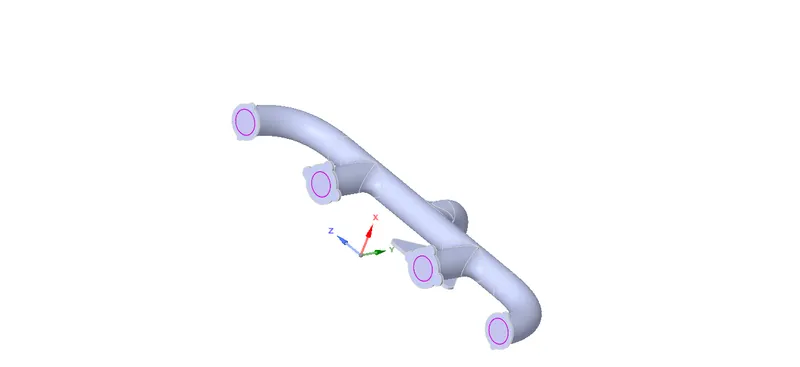
CASE 1 - refined mesh, K-epsillon method

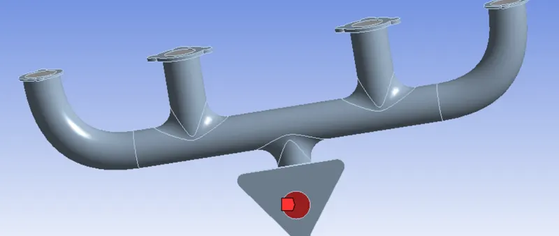
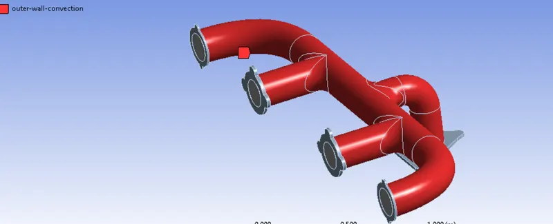
in meshing stage we have named the geometry

inlet :-

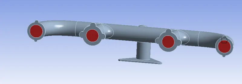
outlet

outer wall convection

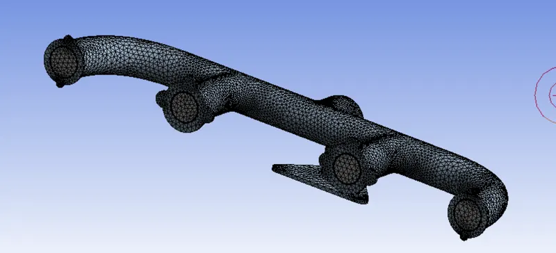
meshing :- (number of nodes 87817, number of elements 249602)

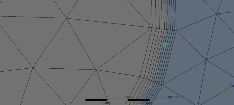
infilation layer

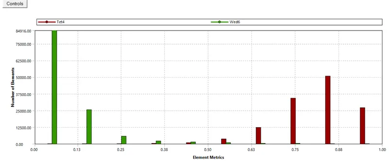
mesh quality :-

Setup -

The first thing we do is setup the boundary conditions which are given below.

• Inlet boundary condition

1. Type: Velocity inlet
2. Velocity magnitude: 5m/s
3. Temperature: 700K

• Outlet boundary condition

1. Type: Pressure outlet
2. Gauge pressure: 0Pa

• Outer wall convection

1. Type: wall
2. Thermal condition: convection
3. Heat transfer coefficient: `20W/M^2K`

The rest boundary condition values are set up as default values in ANSYS-FLUENT

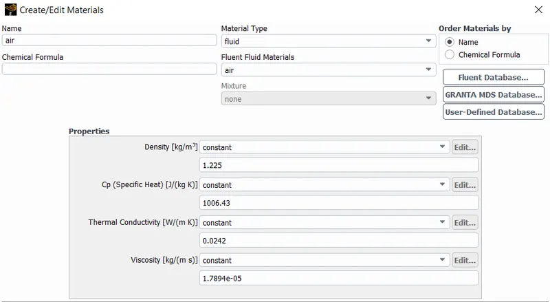
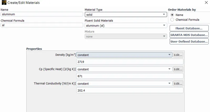
Material properties -

fluid material :-

solid material:-

results :-

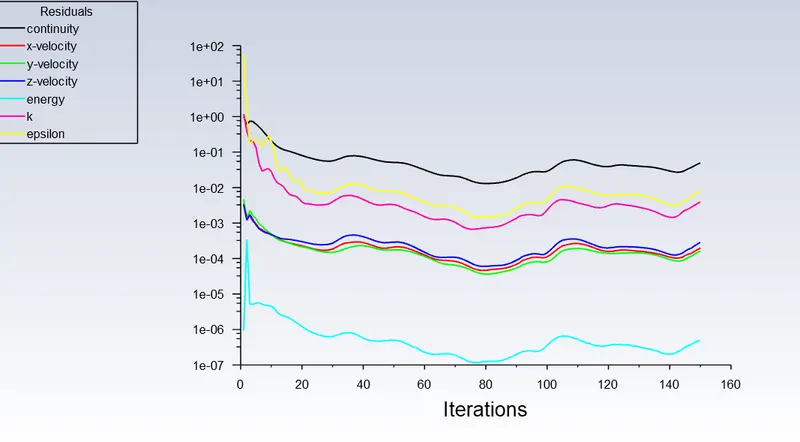
scalar residual plot:-

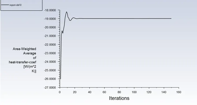
Surface Heat Transfer Coefficient -

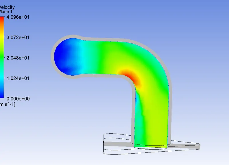
velocity countour

temperature countour

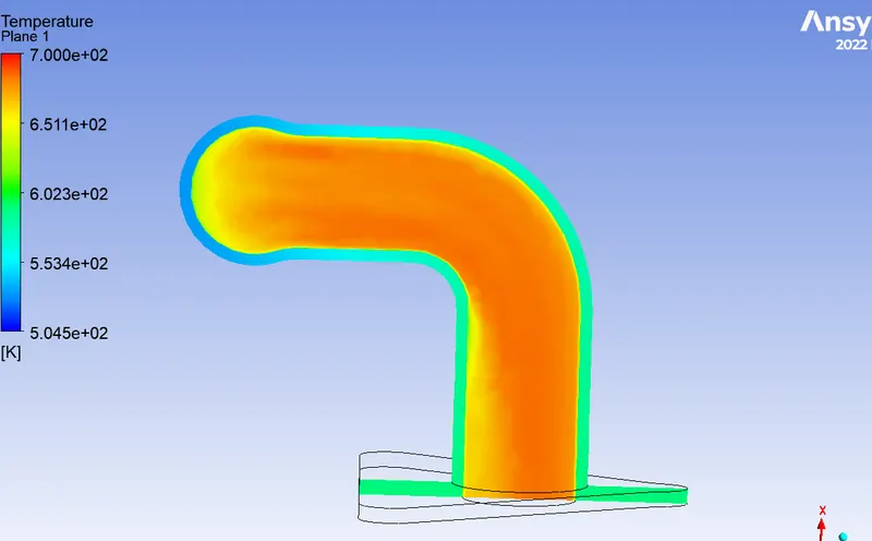
pressure countour

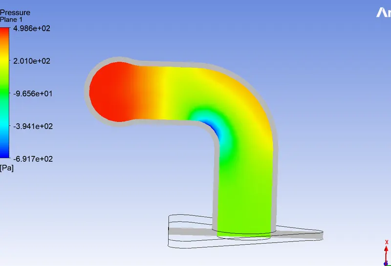
wall heat flux :-

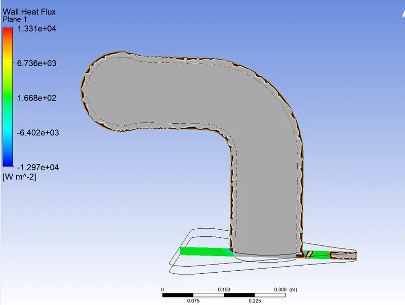
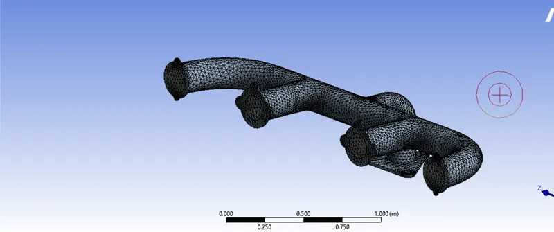
case 2 here the mesh size is refined to much more finer to (184242 nodes ,443281elements )

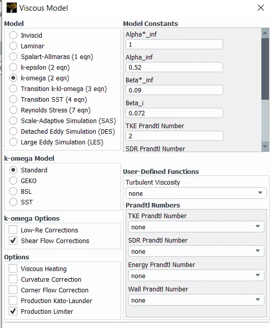
tubulence model :- k-omega-SST model

mesh quality :-

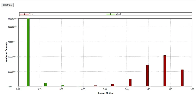
refined mesh :-

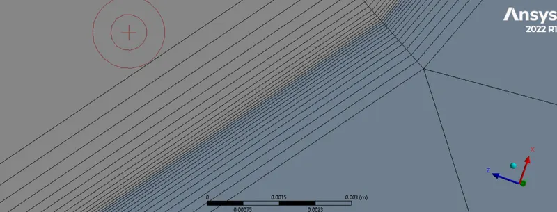
infilation layer with 12 layers

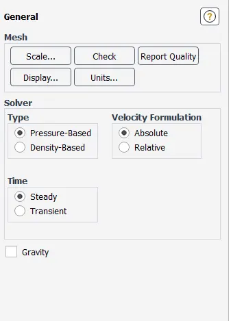
intial set up:-

Material	Fluid type: Air Solid-type: Aluminium
Cell zones	Fluid type: Air Solid-type: Aluminium
Boundaries	Inlet (velocity inlet) Velocity Magnitude 5m/s Temperature – 700K Outlet x (Pressure outlet) Gauge Pressure – 0 pas. Outer-wall-convection -Wall with the thermal condition being convection and heat transfer coefficient All other walls - adiabatic

results ;-

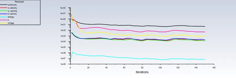
residuals plot:-

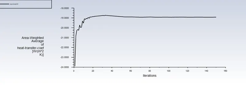
Surface Heat Transfer Coefficient :-

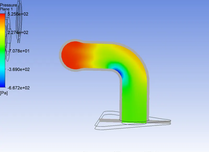
pressure countour:-

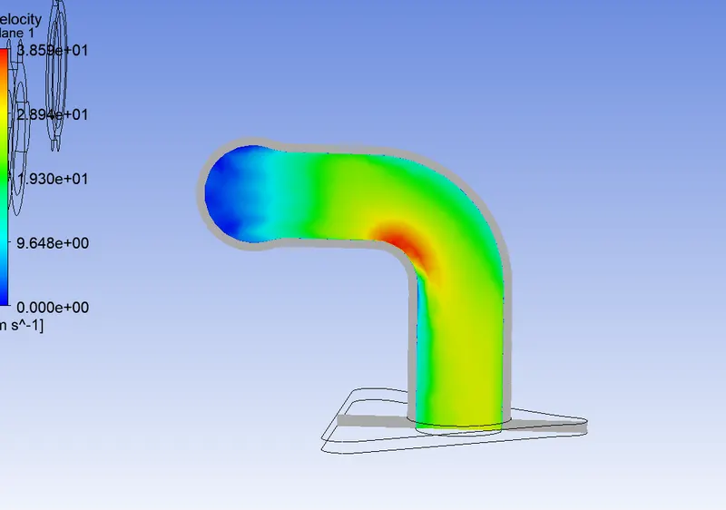
velocity countour :-

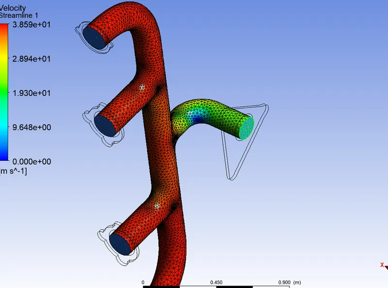
velocity distribution over manifold

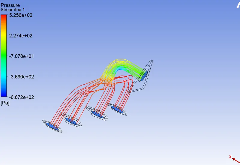
stream line pressure :-

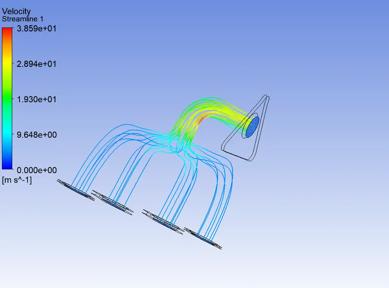
velocity stream line :-

How would you verify if the HTC predictions from the simulations are right?

• The heat transfer coefficient can be verified by comparing the values analytically.
• Analytically heat transfer coefficient can be calculated with the help of Dittus-Boelter equation,

`Nu=0.023Re^0.08Pr^0.4` (when fluid is heated along with the flow)

And `Nu-0.023Re^0.8Pr^0.3` (When fluid is cooled along with the flow)

• In this case, heated fluid is loosing heat (thermal energy) to the walls of the manifold.
• So, `Nu=0.023Re^0.8Pr0.3` is used to calculate the Nusselt number of the respective case.
• Finally the heat transfer coefficient is calculated usimh nusselt number(Nu) = `hL/k`

h = Heat transfer coefficient `W/m^2A`

D_h = hydraulic diameter (m)

K = Thermal conductivity of the fluid `W/mK`

Note: The heat transfer coefficient obtained using analytical means is calculated using the bulk fluid temperature and not with the local wall adjacent temperatures. For numerical validation it is required to take surface heat transfer coefficient in place of wall adjacent heat transfer coeffcient / wall function heat transfer coefficient.

We know that Nusselt no and reynold no are directly propotional and reynold no is proportional to velocity. So HTC is directly proportional to velocity. And from the contours we can see that velocity and HTC are highest at the outlet. So we can predict the results are correct.

Conclusion :

1. Surface heat transfer coefficient was captured smoothly and more acurately in the case of finer mesh.

2. Wall adjacent heat transfer co-efficent was calculated from each cell center which may lead to incorrect result because HTC is depends on the mesh size. So, this method is not suitable for validating.

3. Adding inflation layer gave better results.