Week 4 - CHT Analysis on Exhaust port

CONJUGATE HEAT TRANSFER ANALYSIS

Introduction:

A typical heat transfer analysis involves the calculation of the temperature distribution and flow of heat flux under thermal loads. Both steady-state and transient conditions are simulated. The study of transport phenomenon concerns the exchange of momentum, energy and mass in the form of conduction, convection and radiation. These are the three types of heat transfer involved in various types of materials.

Conjugate Heat Transfer analysis:

A conjugate heat transfer is the simulation between solid and fluid domains by exchanging thermal energy at the interfaces between them. The prediction analysis takes place simultaneously in both solid and fluid boundary. The solid boundary is characterized by stationary material particles, while the fluid boundary is characterized by the moving particles.

Why CHT analysis is used:

A CHT analysis can predict heat transfer through conduction, free or forced convection and radiation heat flows simultaneously between solids and fluids. The wall heat transfer coefficients and local derivatives are calculated within the model, which is an advantage over the empirical calculations.

Where a CHT analysis is used:

The typical application of a CHT analysis is the Heating, ventilation, air-conditioning and refrigeration environment. The key engineering applications include effective heat transfer, energy saving, appropriate heat transfer coefficient formulation etc.

Effective heat transfer in fluids and solids is designed by a CHT analysis. The fluid transports the energy and the solid is used to achieve a separation between different fluids to make sure the fluids don't get mixed during the flow.

Heat loss in engineering applications are simulated to calculate the energy efficiency. The design of thermal insulators, and heat exchangers, power plant parts are based on a CHT analysis.

Procedure:

Step 1: Setting up geometry

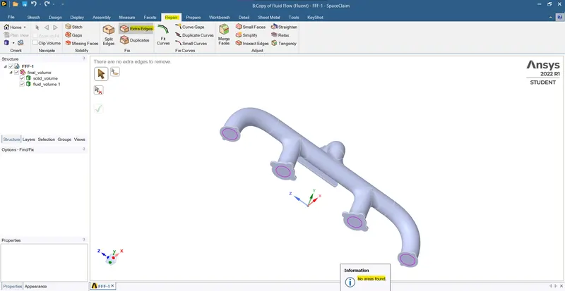
To begin with, the SolidWorks part model is checked for any extra edges in Space Claim Component.

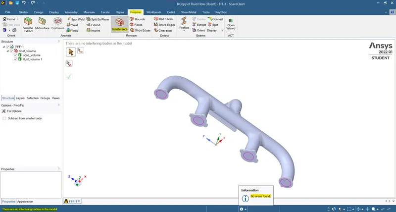
Then the part model is also checked for interferences in the structures.

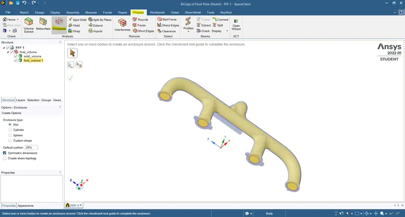
An enclosure is made around the existing model assigned as the solid volume.

The interior volume is assigned the fluid volume, and both the volumes are combined into a single volume.

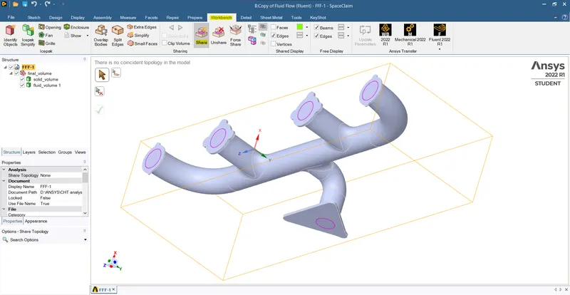
The entire model with two volumes is ensured to share topology.

Step 2: Meshing

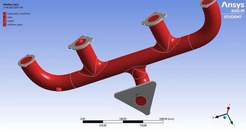
In the Meshing component, the Inlet, Outlet, Inflation Layer and the Outer walls are named.

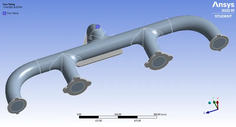
Then a sizing method is introduced for the fluid volume, to preserve the shape features.

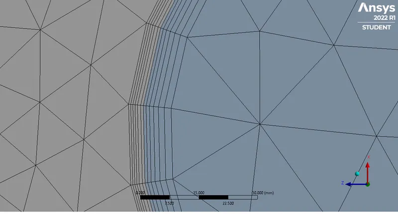
Inflation layer with desired Y+ is added to increase the topology optimization of the mesh cells.

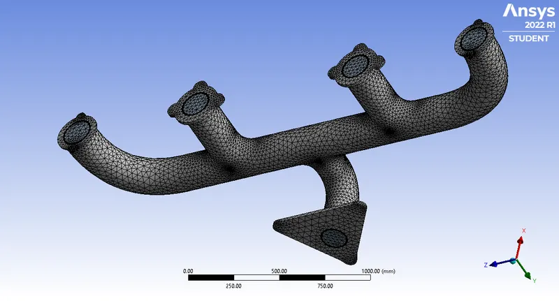
The mesh is generated and checked for quality and interference between the fluid and solid region.

Step 3: Setting up the fluent domain

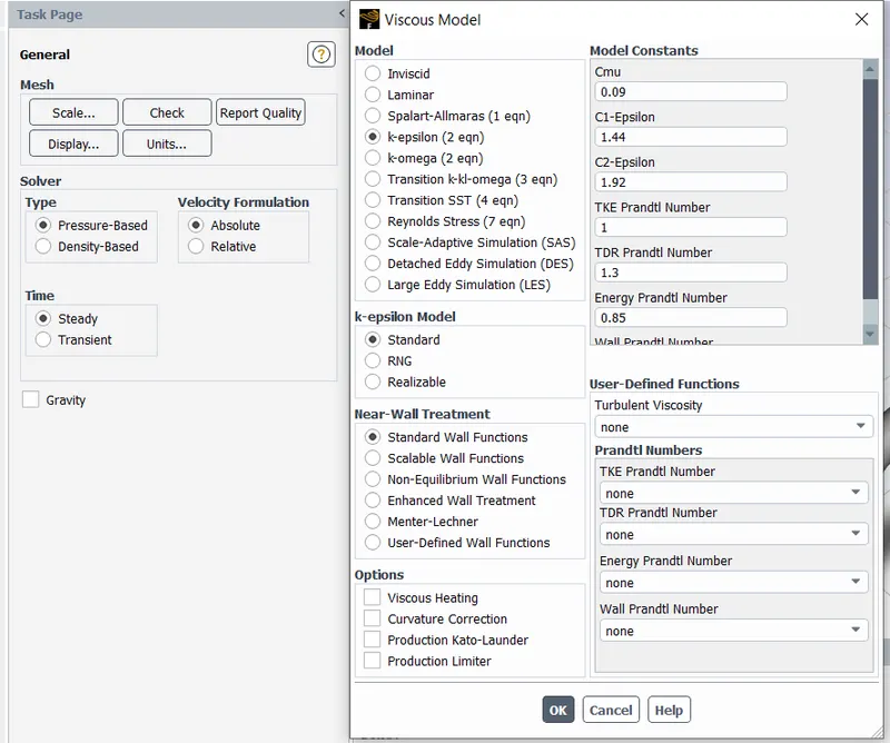
In the Fluent component, the viscous model is selected with appropriate solver type and condition.

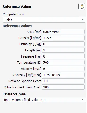
The reference values are computed.

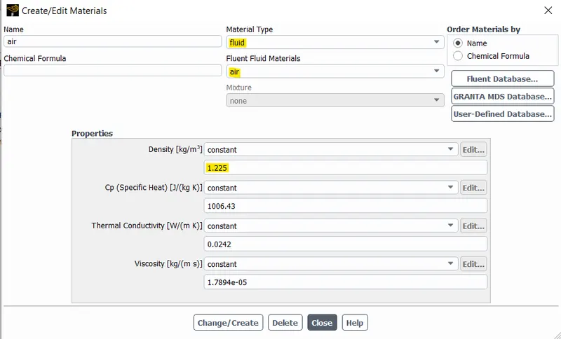
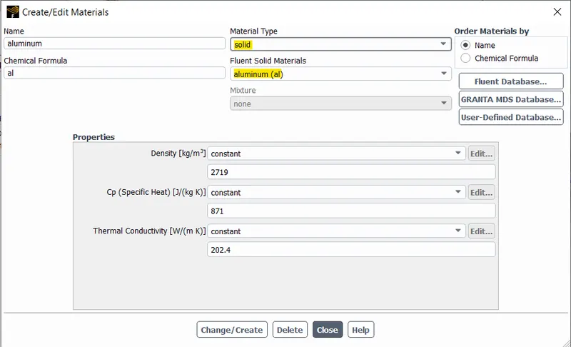
The materials properties are added for fluid and solid types.

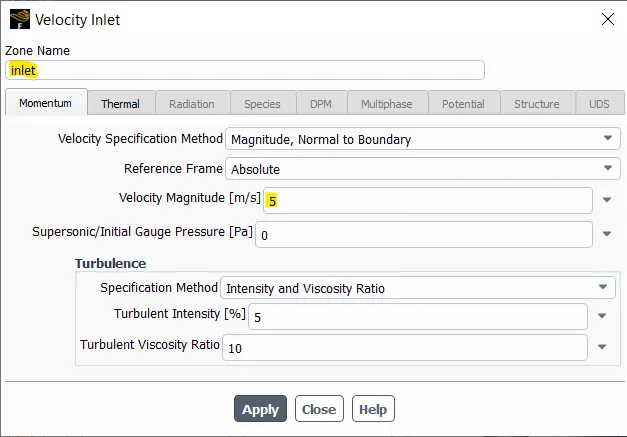
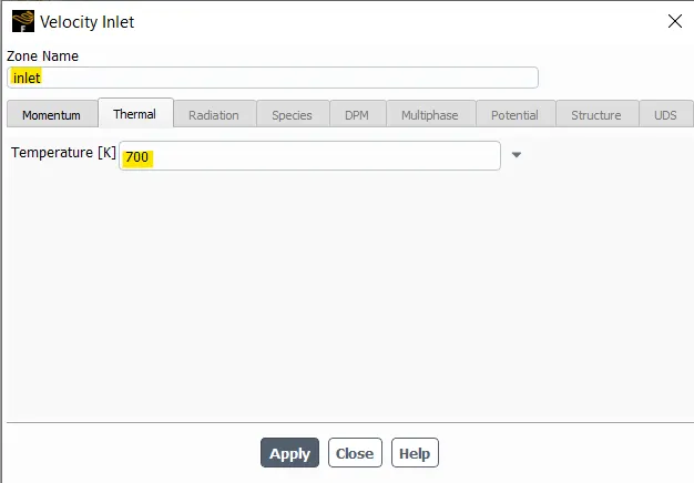
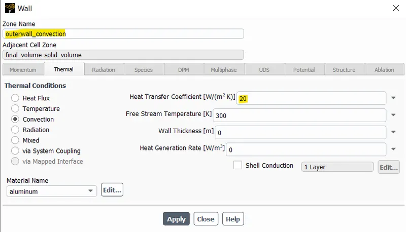
The boundary conditions are set for Inlet, Outlet and Outerwall convection.

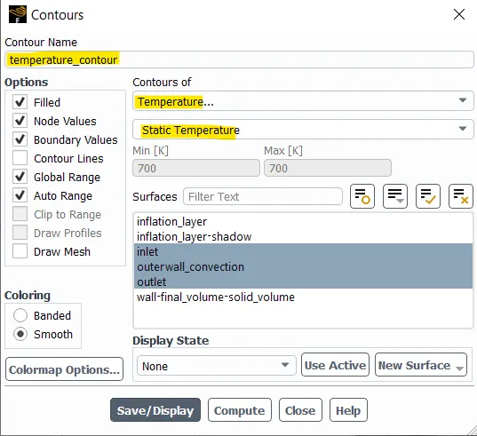
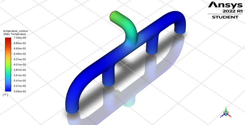
A temperature contour is defined at the specified surfaces.

Step 4: Solution

Hybrid initialization is done and the simulation is run for necessary iterations

A solution animation at the temperature contour is also defined to view the time steps of simulation.

step 5: Post processing

In post processing,

Streamlines starting from Inlet to Outlet is formulated.

An YZ plane is plotted for velocity visualization

Another XY plane is plotted for temperature distribution at Outlet

Results:

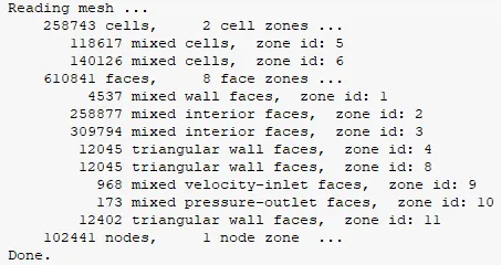
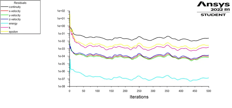
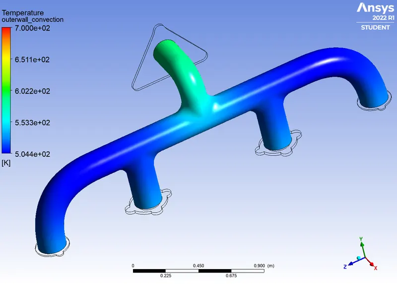
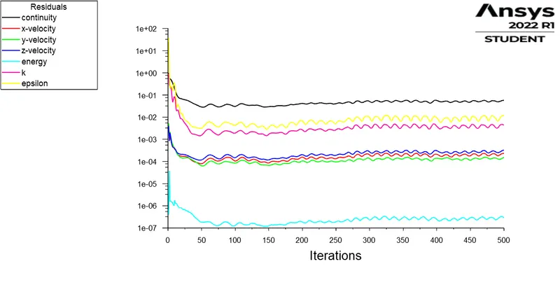
Baseline case: Model: K-Epsilon Standard model Inlet Velocity: 5m/s Inlet temperature: 700K Heat transfer Coefficient: 20 W/m2-K Iterations:500 Mesh Element size: 100mm Sizing: 80mm Inflation layers: 5*0.71*1.2

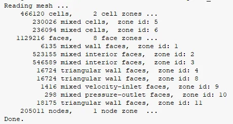
Refined case: Model: K-Epsilon Standard model Inlet Velocity: 5m/s Inlet temperature: 700K Heat transfer Coefficient: 20 W/m2-K Iterations:500 Mesh Element size: 50mm Sizing: 50mm Y+ value: 50 Inflation layers: 10*3.18*1.2

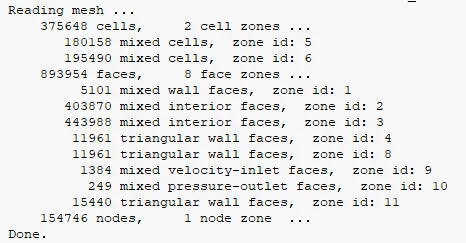
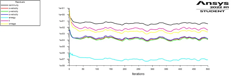
Comparison case: Model: K-Omega SST model Inlet Velocity: 5m/s Inlet temperature: 700K Heat transfer Coefficient: 20 W/m2-K Iterations:500 Mesh Element size: 45mm Sizing: 40mm Y+ value: 2 Inflation layers: 10*0.12*1.2

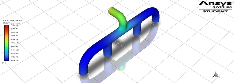Inference:

Streamlines plot

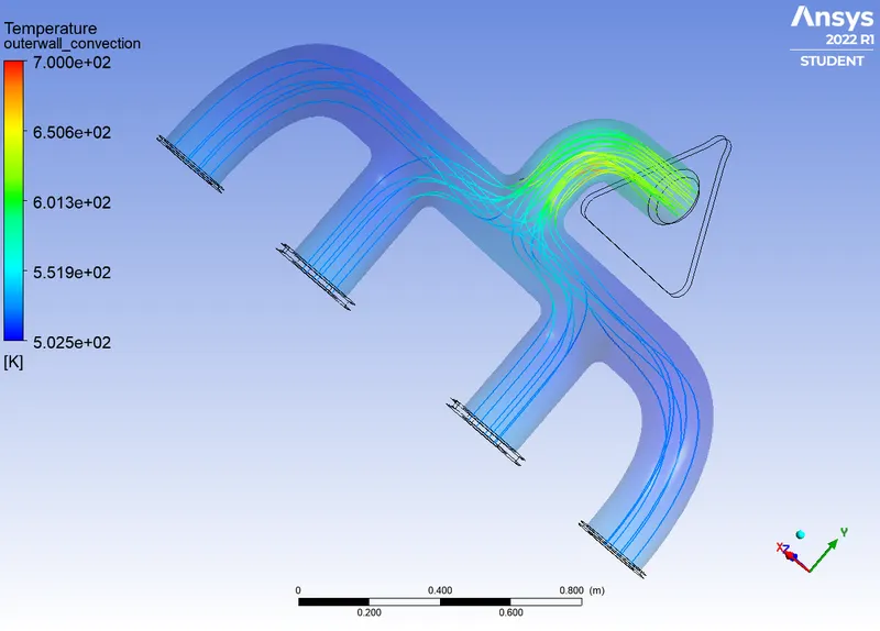
The streamlines plot shows that the particles generate from the inlet and combine at the outlet section, where the velocity increases and the cross-section of the outlet pipe is one of the factor for the increase in velocity.

Velocity plot:

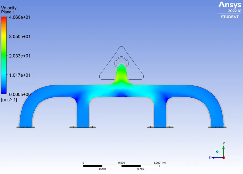
The velocity distribution in the exhaust port is displayed as the contour. It is seen that the velocity at the outlet is around 20m/s., it variates from 5m/s from inlet to 20m/s at the outlet.

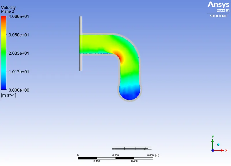
At the 90 degree cross-section of the outlet, the velocity increases to 40m/s due to the minor loss in pipe flow

Temperature plot:

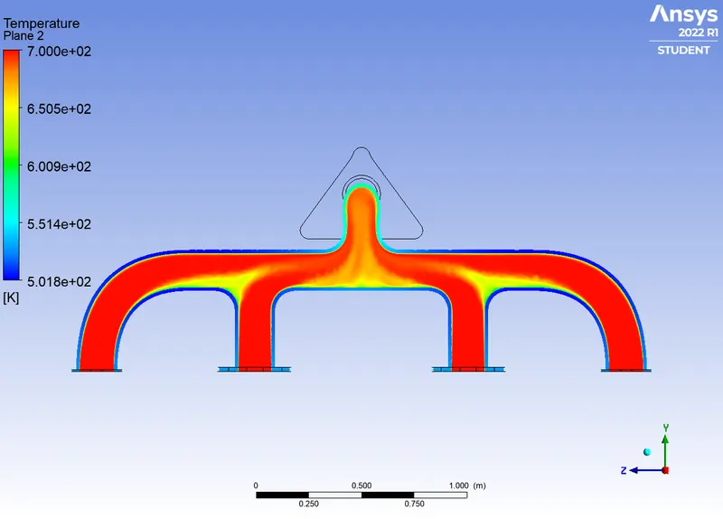
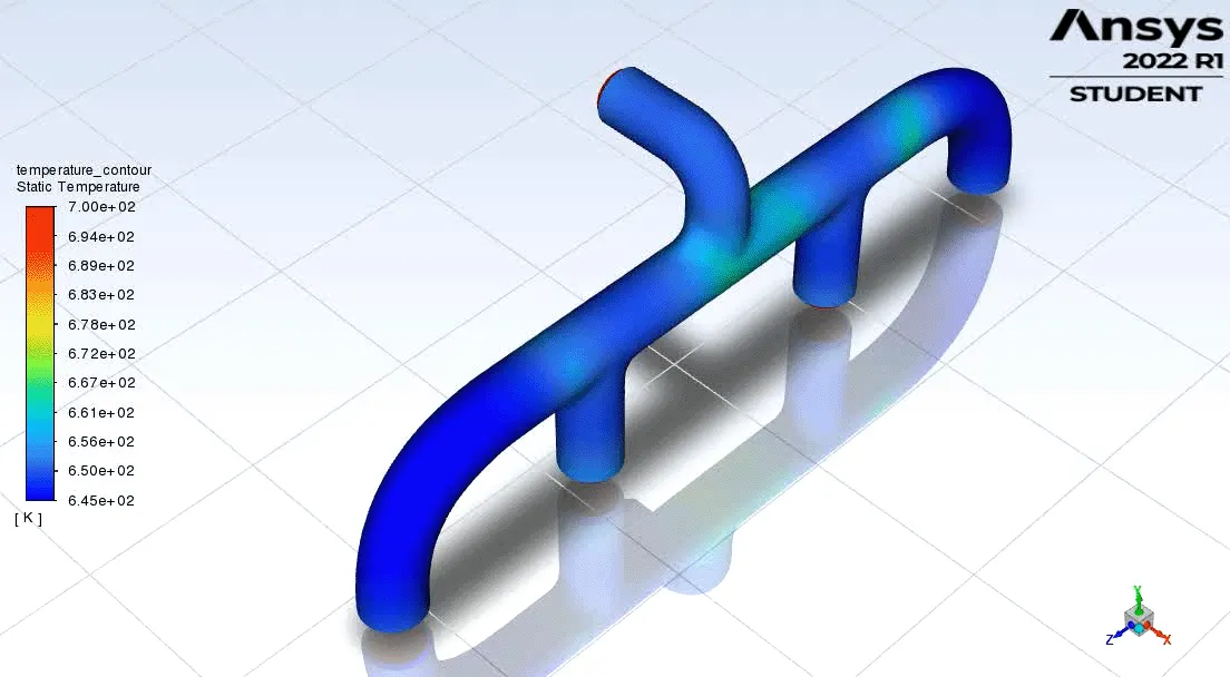
The temperature fluxates from 700K in the inlet to around 650K near the bent wake regions of the internal flow

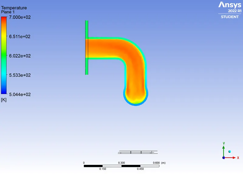
In the outlet, the temperature is around 650K near the walls and 680K in the center of the flow

Wall heat transfer coefficient:

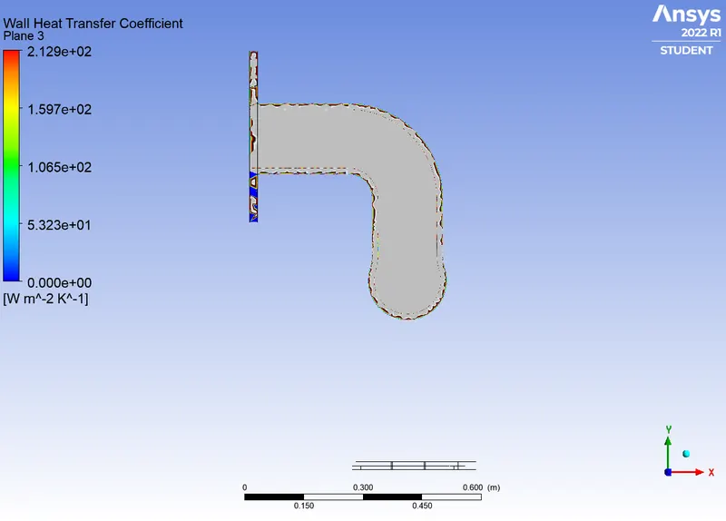
In the outlet, the wall heat transfer coefficient is simulated to a value of 200 `(W)/((m^2) K)`

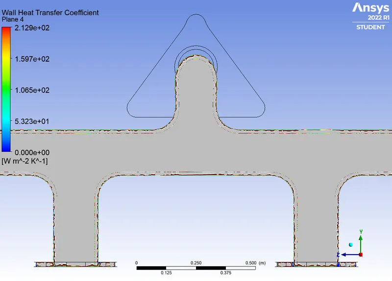
In the inlet, the wall heat transfer coefficient is around 200 `(W)/((m^2) K)` near the walls, and around 150`(W)/((m^2) K)` in wall adjacent layers.

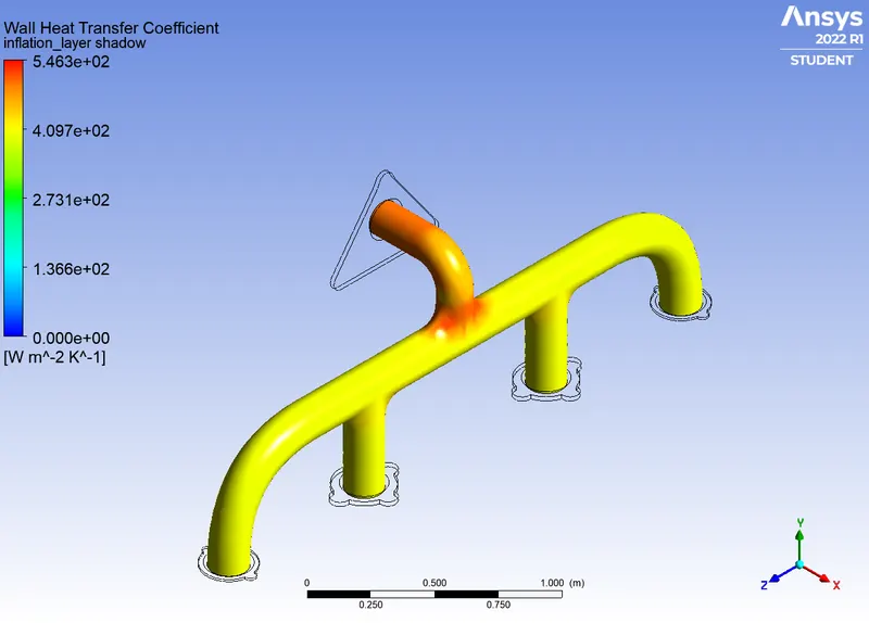
The wall heat transfer coefficient value is between 400`(W)/((m^2) K)` to 500 `(W)/((m^2) K)`

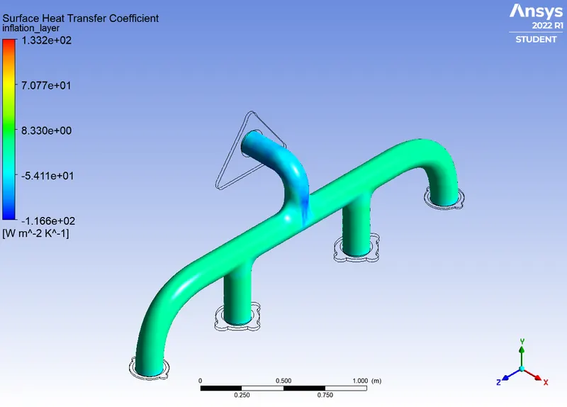
Verifying the accuracy of Heat Transfer Coefficients from the simulation:

Arriving from the Bernoulli's mass conservation principle, mass is conserved in our model. The mass flow rate from the inlet is equal to the mass flow rate at the outlet. Hence as mass flow rate is balanced, the velocity increases for an incompressible flow which increases the Reynolds number.

Introducing Nusselt number, Nu=f(Re,pr) for forced convection

Nusslet number is the ratio of Convective heat transfer to conductive heat transfer.

The relations `Nu=h/((k/L)` and `Nu=0.023Re^(4/5).Pr^(n)` gives the relations between nusselt number, heat transfer coefficient and reynolds number.

Therefore from the relations, as velocity increases by way of increasing the reynolds number, the heat transfer coefficient also increases, which is in accordance with the simulation result.

Factors influencing the accuracy of prediction:

• The important factor influencing the accuracy is the shadow wall which is created automatically by the fluent module, and helps in maintaining a distinguished boundary between fluid and solid interface, thereby increasing efficiency of a CHT prediction.
• The mesh quality with the inflation layers increases the accuracy, while the body sizing method of the solid volume and the sharing of topology in the mesh adds refinement to the prediction.
• Appropriate Y+ value designation adds up to accuracy, as it increases the mesh quality near the walls, which is very useful in the case of a CHT analysis.
• The number of inflation layers also adds up to the near wall accuracy and so increases accuracy.
• The solver selected, turbulence model and the also has impacts on the accuracy

Conclusion:

Thus the Conjugate heat transfer analysis is done on an exhaust port and is simulated with two different models to verify the heat transfer coefficient and the accuracy predicted is proved to be in accordance with the simulation results and the factors for the accuracy are also derived.