Week 4 - CHT Analysis on Exhaust port

Aim –

T o study the Phenomena of conjugate heat transfer. And flow analysis through engine exhaust pipe.

Introduction –

Conjugate Heat Transfer (CHT) –

1. It is analysis type allows for the simulation of heat transfer between solidand fluid domains by exchanging thermal energy at the interfaces between them.
2. Typical applications of CHT - heat exchangers, cooling of electronic equipment, and general-purpose cooling and heating systems.
3. In solids the heat transfer take place through conduction and in fluid it is due to the convection.

Why CHT is used-

1. It is basically used to understand the heat transfer mechanism and temperature distribution at both domains.
2. Its help to understand the velocity contours for sharp bends and pipe end.
3. With help of CHT analysis we can see the coefficient of the heat transfer variation. which further help to analysis the life of the components.

CHT Applications-

It is basically help to do study of IC engine components, Cooler, HVAC systems etc.

How would you verify if the HTC predictions from the simulations are right? On what factors does the accuracy of the prediction depend on?

1. The Nusselt number (Nu) is the ratio of convective to conductive heat transfer at a boundary in a fluid.
2. A Nusselt number of values one represents heat transfer by pure conduction.

where h - convective heat transfer coefficient of the flow,

L - characteristic length

k - thermal conductivity of the fluid.

Geometry –

Load the geometry in space claim.

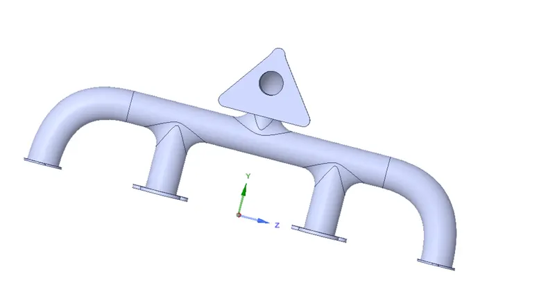
After loading the geometry in the space claim. Separate the fluid volume by volume extraction tap in prepare tab . Then enable the sharing in share the topology to prevent any intersection error of mesh on edges.

Meshing –

Meshing is done in Ansys mesh in fluent module. Before doing the mesh define the inlet, outlet and convection body as named selection.

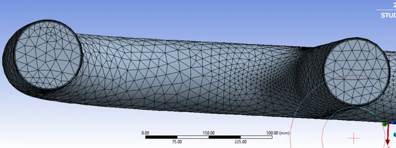
Generate the normal mesh.

For inflation layer, select the inner faces and provide the total thickness to the layer.

Element size for the outer body to be set as – 20mm

No of cells - 205034 cells

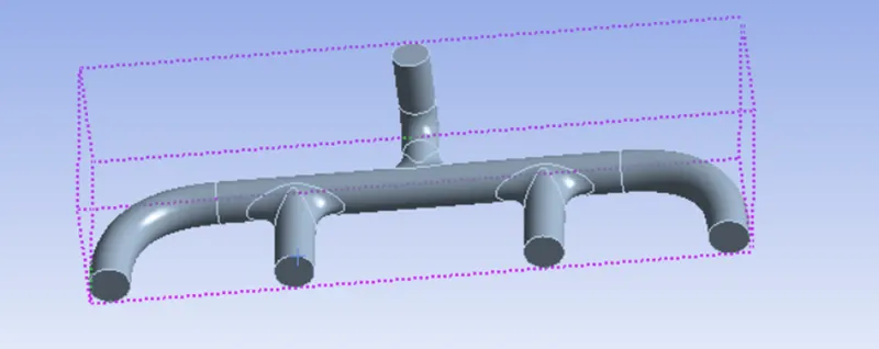
Setup

Solver Type – Pressure based and steady state

velocity formation – Absolute

Model – K-Epsilon

Fluid type – Air

Solid type - Aluminium

Boundary Condition -

Inlet velocity – 5 m/s , Temperature – 700K

Outlet – Type – Pressure outlet

Outer wall convection – wall type, HTC- 20

Initialization – Hybrid

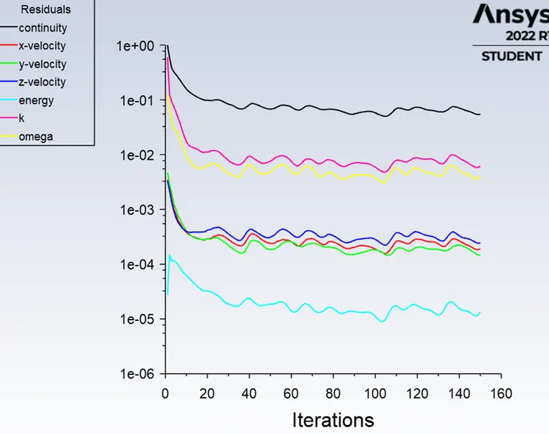
No of iteration – 150

Residual plot

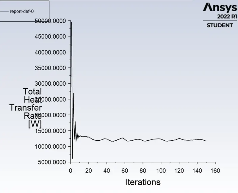
Total heat transfer rate –

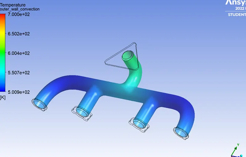
Temprature contour for outer wall -

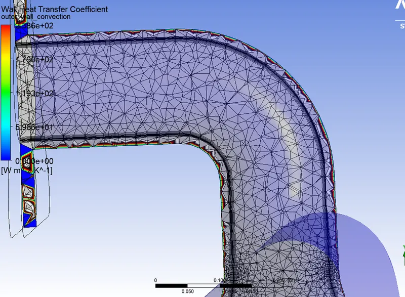
Heat trabsfer coffcient -

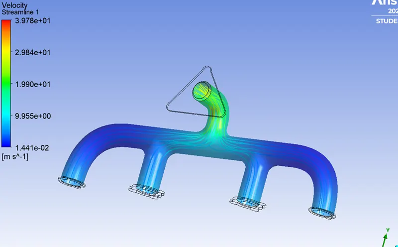
Velocity contour with streamlines -

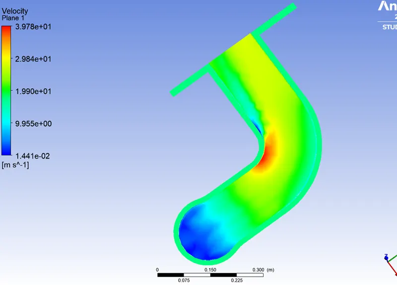
Velocity contour for outlet bend pipe -

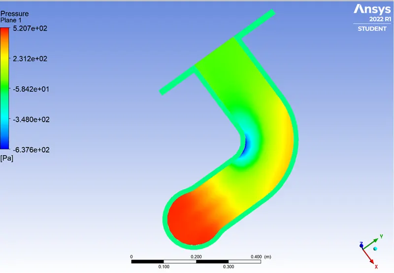
Pressure contour for outlet bend pipe -

Conclusion as per post results –

1. It is observed that the velocity streamline is more at the outlet due to mass conservation at the end of flow.
2. Velocity at all the inlet is same.
3. At the outlet bend it is noticed that velocity is high, so at that point Reynolds number will be high and which indicate the Nusselt number will al so be more.
4. Due to the high Nusselt number the coefficient of the heat will be more where velocity is high.
5. Finer the mesh better the result we get. As we increase the mesh quality at the interface it gives better view to see the change of velocity and pressure along the surface.Thats why y+ has to define as per the solver model .
6. Higher the HTC shows the area where high temperature exist due to heat transfer.