Week 4 - CHT Analysis on Exhaust port

AIM: To study the Conjugate Heat Transfer Analysis using the Exhaust Port.

OBJECTIVE:

• Give a brief description of why and where a CHT analysis is used. • Maintain the y+ value according to the turbulence model and justify the results.

• Calculate the wall/surface heat transfer coefficient on the internal solid surface & show the velocity & temperature contours in appropriate areas.

• How would you verify if the HTC predictions from the simulations are right? On what factors does the accuracy of the prediction depend?

CONJUGATE HEAT TRANSFER ANALYSIS.

The Conjugate Heat Transfer (CHT) analysis type allows for the simulation of heat transfer between solid and fluid domains by exchanging thermal energy at the interfaces between them.

The fluid usually plays the role of energy carrier on large distances. Forced convection is the most common way to achieve a high heat transfer rate. In some applications, the performances are further improved by combining convection with phase change (for example liquid water to vapour phase change).

Even so, solids are also needed, in particular, to separate fluids in a heat exchanger so that fluids exchange energy without being mixed.

Typical applications of this analysis type exist as, but are not limited to, the simulation of heat exchangers, cooling of electronic equipment, and general-purpose cooling and heating systems.

PROCEDURE:

GEOMETRY.

• In the space claim setup, we are setting up the CAD model geometry of the exhaust port which is already present in our system.
• Change the units to meters in the space claim and go to prepare Extract the volume by selecting the inner edges of the solid body.
• then go to repair remove the extra edges if any, and then go to the workbench and click on the share command and then enable the share topology.

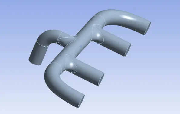
The geometry of the Exaust port is as below

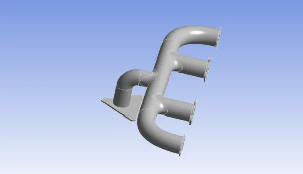
The fluid domain

MESH.

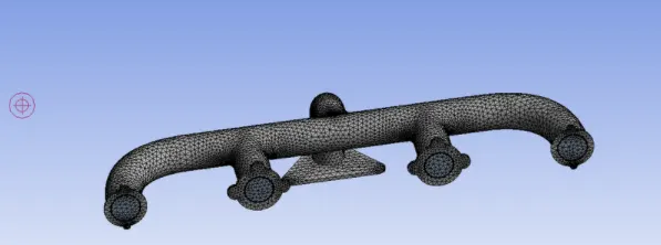
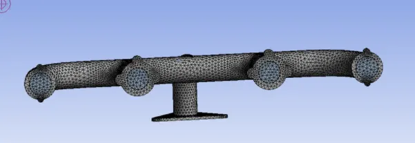
• We are creating the baseline mesh and then we are going to refine the mesh.
• in the mesh setup, we are using the named selection command to name the boundaries by selecting the respective face or body selection option.
• Then go to Mesh insert>Sizing>Select solid body>assign the element size, and then in the sizing> Advance> curvature capture>yes.
• Then, Mesh >Inflation>Use Automatic inflation>All faces in chosen, and named selection>Select inflation layer, Inflation option>Total thickness, assign the number of layers, growth rate, and the maximum thickness.
• Now, generate the mesh and observing the elements and nodes in the statistics.

SETUP.

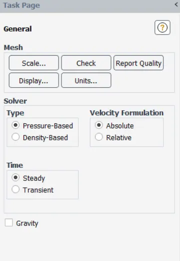
• In the setup, we are setting up the physics of the simulation. Setup>physics>general setting>solver type>pressure based.
• Setup>physics>general setting>time>steady.
• model>check energy.
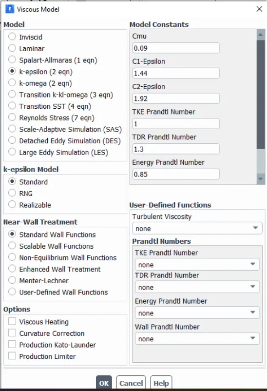
• physics model>viscous model>K-epsilon or K-Omega, in the baseline I have taken the K-epsilon model and for refined mesh, i have taken K-Omega, SST model.
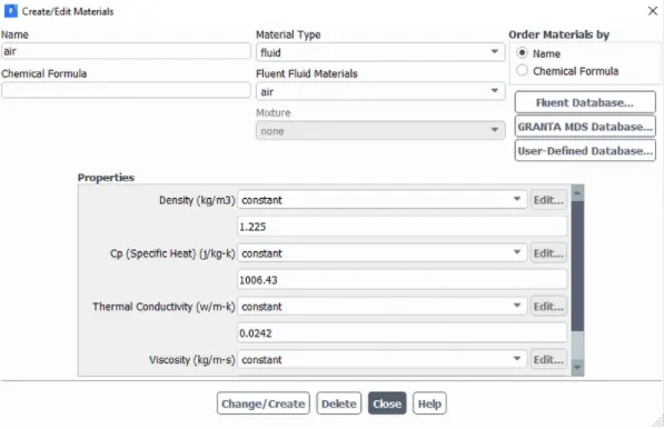
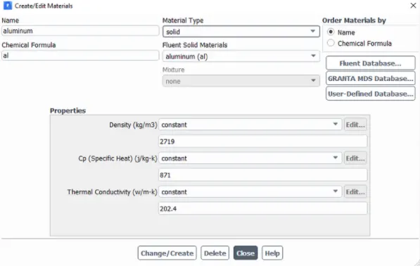
• physics> material>material type>fluid/solid. physics> material fluent fluid material air/aluminium.
• physics> material properties> I have taken the default values here.
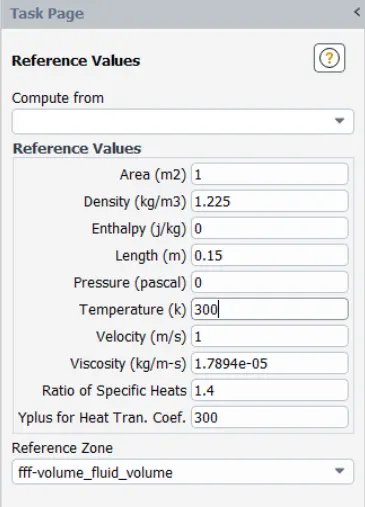
• physics>zones>boundaries>inlet> velocity as 5m/s and in thermal properties temperature as 700k and rest of all are default values.
• physics zones>boundaries>outlet pressure as 0.
• physics zones>boundaries>outer convection wall>thermal>convection, HTC as 20 w/m^2k, free stream temperature as 300k.
• Setup>solution>report>residuals>uncheck all the absolute convergence criteria and using the hybrid method initialize the simulation.
• and run the simulation for the required number of iterations.

SOLUTION.

In the solution, we can obtain all the simulation reports and plots.

RESULTS.

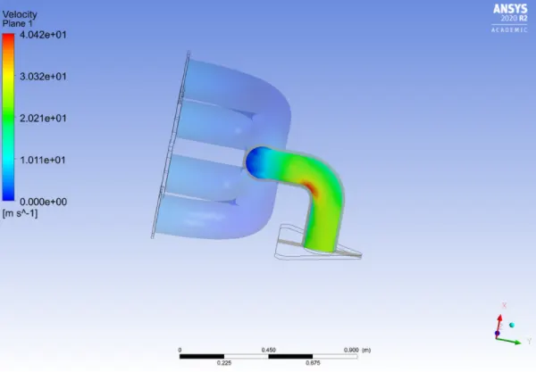
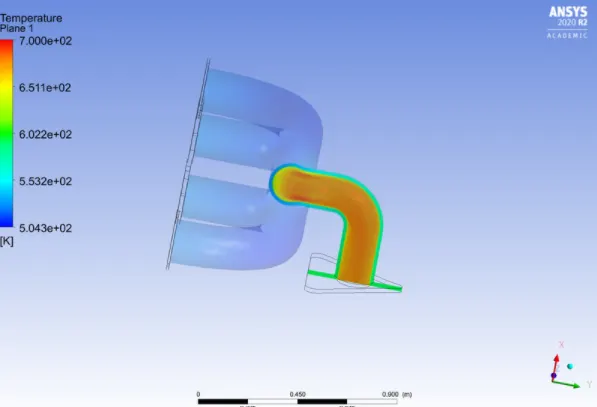
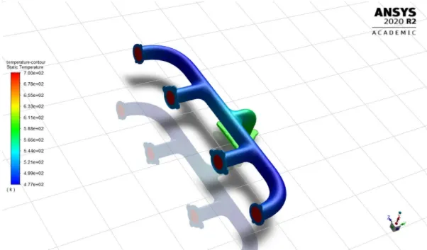
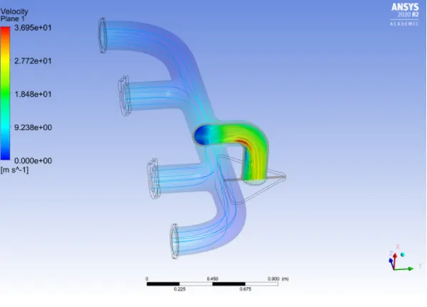
In the CFD-post we can get the velocity and temperature planes and also the streamline flow diagram for the CHT analysis.

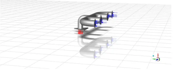
In the below diagram we can observe the 4 inlets of the exhaust port which has blue coloured arrows and the outlet which has the red coloured arrows and the outer solid body.

RESULT

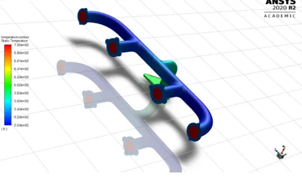
tempearture contour

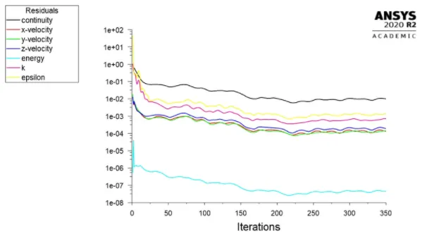
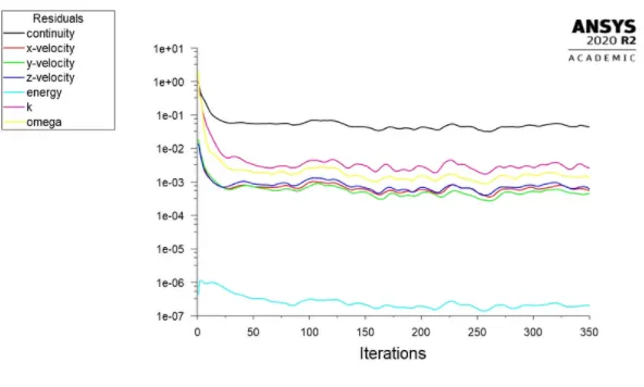
Residual

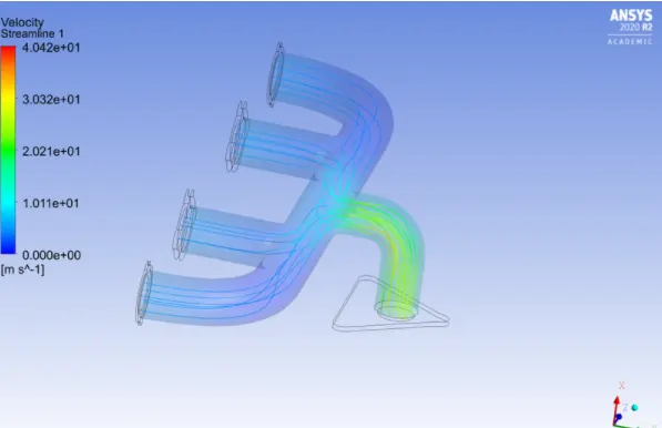
Velocity streamline contour

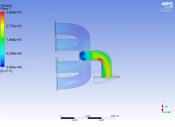
Velocity contour plane

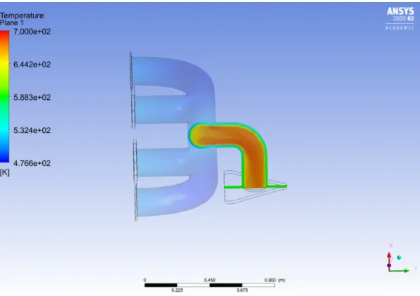
Temperature contour plane

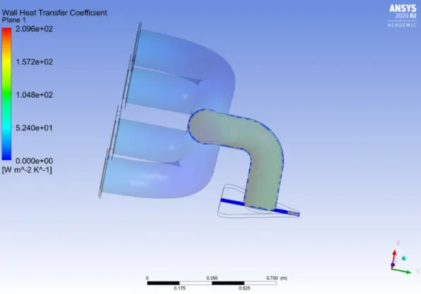
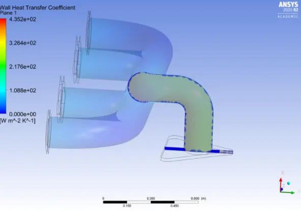
Wall heat transfer coefficient

2.Refined mesh simulation

Y-plus: 3

Inflation Maximum thickness: 1.24mm

Viscous Model: K-epsilon

Inlet velocity: 5 m/s.

Inlet temperature: 700K.

Outlet gauge pressure: 0.

Heat transfer coefficient: 20 w/m^2-k.

Fluent material: Air.

Density of air: 1.225 kg/m^3.

Dynamic viscosity of air: 0.000017894 kg/m-s

Temperature contour

Residual plot

Velocity streamline flow

Velocity contour plane

Temperature contour plane.

Wall heat transfer coefficient.

HEAT TRANSFER COEFFICIENT VERIFICATION.

Heat Transfer coefficient at boundary surface is often calculated using Nusselt number. Hence to verify the HTC obtained from the CHT analysis we first need to calculate the theoretical value of the Nusselt number.

For a turbulent flow inside a smooth pipe, Nu number is given by Dittus-Boelter equation.

(Nu)p=0.023 (Re)^4/5 *(Pr)^n ----1

Also,

Nu=hL/k= ---2 k

D = Diameter of the circular duct,

Pr Prandtl number,

n = 0.4 for the fluid being heated, and n = 0.3 for the fluid being cooled.

Nu = Nusselt Number

Re Renolds number

Hence, using the value of Nu from (1) we can find the value of the heat transfer coefficient, h from equation (2) and verify it with the actual results obtained from the above simulations.

By examining the velocity contours at the plane we can understand that there is a high velocity at the bent which implies a high Reynold number. From the above relation, we can say that as Re increases Nu increases as well, which in turn increases the heat transfer coefficient.

Factors affecting the accuracy of prediction from simulations are

• Inflation layer - It increases the quality of mesh near the boundary interface and it can capture smooth plots of heat transfer coefficient.
• Grid size and shape -The grid size as it decreases the quality of the mesh will increase and also the shape of the mesh also matters and gives more accurate result.
• Setting share topology - Mesh should be conformal for smooth transferring of mesh in different zones

Conclusion

1. The results are more accurate in the second and third case as compared with the first case due to the mesh refinement.
2. There is no change in temperature difference in all the cases but the change in minimum temperature, it is in the second and third case because of mesh refinement.
3. The wall coefficient heat transfer also increases in the second and third case.
4. The velocity and hence the Reynolds number is higher at the outlet. Due to that, the heat transfer and temperature is higher.
5. The heat transfer coefficient is higher between fluid and solid at the outlet pipe, because the velocity of the fluid is higher