Week 7 - Simulation of a 1D Super-sonic nozzle flow simulation using Macormack Method

Motivation

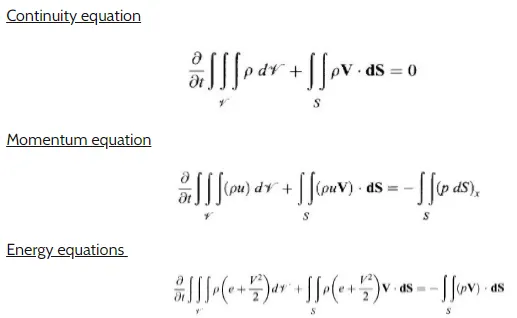
So far we have learnt some ideas on Governing equations, their forms (w/o knowing their actual means), FDM, Consistency of a Numerical scheme, Discretization (FDM), Time integration, Stability and more or less few. Now we put all of these together.

Governing equations

In Conservative form we consider control volume is staionary whereas in Non-Conservative form CV is moving. Both are mathematically same and can easily converted into another easily and excatlty. They have difference only in numerical discretization.

1D supersonic nozzel flow

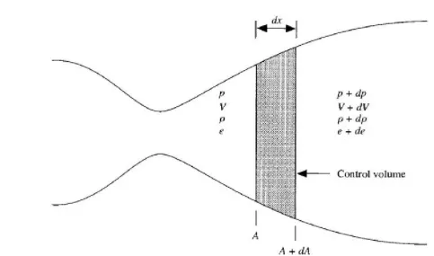
The convergence(subsonic) section connected with reservoir, here mach number is less than one. At throat area, the thermodynamic properties will become critical property as Mach number equal to 1. The sonic flow at the throat means that the local velocity at this point is equal to the local speed of sound and at divergence section(supersonic) the flow expands isentropically to supersonic speed at the nozzle exit. The corresponding notations are clearly written in the figure itself.

The flow is locally subsonic in the convergence section of the nozzle, sonic at the throat and supersonic at the divergence section.

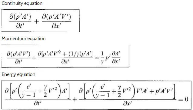
The governing continuity, momentum and energy equation for the quasi 1D steady isentropic flow can be expressed as

Non conservative form:

Conservative form:

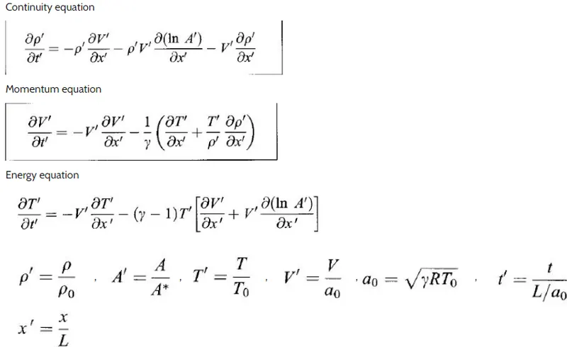
Using Maccormack method, we can solve both of these sets of equations. In this method we use two rounds of iteration namely predictor and corrector steps which solve the premitive variables using FDS and BDS respectively, then we use arthimetic mean of both results. Following are the sets of Matlab programs with defined initial and boundary conditions as per Anderson book with separate functions for Non-conservative and conservative terms.

Main code:

clear all
close all
clc

%%Discretization
L=3;
n=31;
x=linspace(0,L,n);
dx=x(2)-x(1);
throat=(n+1)/2;
% profile of nozzel and parameters
a=1+2.2*(x-1.5).^2;

%fluid properties
gama=1.4;
C=0.5;
nt=1400;

tic
[m_Nc,m_Nc_t,M_Nc,M_Nc_t,rho_Nc,rho_Nc_t,P_Nc,P_Nc_t,T_Nc,T_Nc_t,V_Nc,V_Nc_t]=NonConservative(x,n,dx,gama,nt,a,C,throat);
t_non_conservative=toc;
fprintf('time consumed for non conservative form=%d\n',t_non_conservative);

tic
[m_c,m_c_t,M_c,M_c_t,rho_c,rho_c_t,P_c,P_c_t,T_c,T_c_t,V_c,V_c_t]=Conservative(x,n,dx,gama,nt,a,C,throat);
t_conservative=toc;
fprintf('time consumed for conservative form=%d',t_conservative);

%Grid dependence test
% % Calcualtinng primitive values at throat
terms={'Nondimensional density';'Nondimensional temperature';'Nondimensional pressure';'Mach number'};
exact_solution=[0.634;0.8333;0.528;1];
conservative_terms=[rho_c(throat);T_c(throat);P_c(throat);M_c(throat)];
non_conservative_terms= [rho_Nc(throat);T_Nc(throat);P_Nc(throat);M_Nc(throat)];
table(terms,exact_solution,conservative_terms,non_conservative_terms)

figure(3)
plot(x,m_Nc)
hold on
plot(x,m_c)
title('comparison of non dimensional mass flow rates')
legend('Non_conservative form', 'conservative form')
xlabel('x/L')
ylabel('Nondimensional mass flow rate')

figure(4)
subplot(4,1,1)
plot(x,M_Nc)
xlabel('x-axis')
ylabel('Mach number')
subplot(4,1,2)
plot(x,rho_Nc)
xlabel('x-axis')
ylabel('Density ratio')
subplot(4,1,3)
plot(x,P_Nc)
xlabel('x-axis')
ylabel('Pressure ratio')
subplot(4,1,4)
plot(x,T_Nc)
xlabel('x-axis')
ylabel('Temperature ratio')
subtitle('Solution for Non conservative form at steady state')

figure(5)
subplot(4,1,1)
plot(x,M_c)
xlabel('x-axis')
ylabel('Mach number')
subplot(4,1,2)
plot(x,rho_c)
xlabel('x-axis')
ylabel('Density ratio')
subplot(4,1,3)
plot(x,P_c)
xlabel('x-axis')
ylabel('Pressure ratio')
subplot(4,1,4)
plot(x,T_c)
xlabel('x-axis')
ylabel('Temperature ratio')
subtitle('Solution for Conservative form at steady state')

Function for Non conservative:

% Non conservative function
function[m_Nc,m_Nc_t,M_Nc,M_Nc_t,rho_Nc,rho_Nc_t,P_Nc,P_Nc_t,T_Nc,T_Nc_t,V_Nc,V_Nc_t]=NonConservative(x,n,dx,gama,nt,a,C,throat);
% initial condition along x
rho_Nc=1-0.3146.*x;
T_Nc=1-0.2314.*x;
V_Nc=(0.1+1.09*x).*T_Nc.^0.5;
throat=16;
%time step

% dt(i)=C.*(dx./((T(i)).^0.5+V(i)));
Dt=min(C*(dx./(T_Nc.^0.5+V_Nc)));
for k=1:1400
    % values at time t
    rho_old=rho_Nc;
    T_old=T_Nc;
    V_old=V_Nc;
    %a_old=a;
    
    % maccormack method
    for j=2:n-1
        dvdx=(V_Nc(j+1)-V_Nc(j))/dx;
        dlog_a_dx=(log(a(j+1))-log(a(j)))/dx;
        drhodx=(rho_Nc(j+1)-rho_Nc(j))/dx;
        dTdx=(T_Nc(j+1)-T_Nc(j))/dx;
        
        % continity equation
        drhodt_p(j)=-(rho_Nc(j)*dvdx)-(rho_Nc(j)*V_Nc(j)*dlog_a_dx)-(V_Nc(j)*drhodx);
        % Mommentum equation
        dvdt_p(j)=-V_Nc(j)*dvdx-(1/gama)*(dTdx+(T_Nc(j)/rho_Nc(j))*(drhodx));
        % Energy equation
        dTdt_p(j)=-V_Nc(j)*dTdx-(gama-1)*T_Nc(j)*(dvdx+(V_Nc(j)*dlog_a_dx));
        
        % solution update at time step 't+dt'
        rho_Nc(j)=rho_Nc(j)+drhodt_p(j)*Dt;
        V_Nc(j)=V_Nc(j)+dvdt_p(j)*Dt;
        T_Nc(j)=T_Nc(j)+dTdt_p(j)*Dt;
    end
    
    % corrector step
    for j=2:n-1
        dvdx=(V_Nc(j)-V_Nc(j-1))/dx;
        dlog_a_dx=(log(a(j))-log(a(j-1)))/dx;
        drhodx=(rho_Nc(j)-rho_Nc(j-1))/dx;
        dTdx=(T_Nc(j)-T_Nc(j-1))/dx;
        
        % continity equation
        drhodt_c(j)=-(rho_Nc(j)*dvdx)-(rho_Nc(j)*V_Nc(j)*dlog_a_dx)-(V_Nc(j)*drhodx);
        % Mommentum equation
        dvdt_c(j)=-V_Nc(j)*dvdx-(1/gama)*(dTdx+(T_Nc(j)/rho_Nc(j))*(drhodx));
        % Energy equation
        dTdt_c(j)=-V_Nc(j)*dTdx-(gama-1)*T_Nc(j)*(dvdx+(V_Nc(j)*dlog_a_dx));
        
    end
    % Arithmatic mean of pde
    drhodt_avg=0.5*(drhodt_p+drhodt_c);
    dvdt_avg=0.5*(dvdt_p+dvdt_c);
    dTdt_avg=0.5*(dTdt_p+dTdt_c);
    
    % Final update solution
    for i=2:n-1
        rho_Nc(i)=rho_old(i)+drhodt_avg(i)*Dt;
        V_Nc(i)=V_old(i)+dvdt_avg(i)*Dt;
        T_Nc(i)=T_old(i)+dTdt_avg(i)*Dt;
    end
    
    % BC
V_Nc(1)=2*V_Nc(2)-V_Nc(3);
V_Nc(n)=2*V_Nc(n-1)-V_Nc(n-2);
rho_Nc(n)=2*rho_Nc(n-1)-rho_Nc(n-2);
T_Nc(n)=2*T_Nc(n-1)-T_Nc(n-2);
%calculating
m_Nc=rho_Nc.*V_Nc.*a;
M_Nc=V_Nc./(T_Nc.^0.5);
P_Nc=rho_Nc.*T_Nc;

% flow parameter defining
P_Nc_t(k)=P_Nc(throat);
T_Nc_t(k)=T_Nc(throat);
V_Nc_t(k)=V_Nc(throat);
rho_Nc_t(k)=rho_Nc(throat);
m_Nc_t(k)=m_Nc(throat);
M_Nc_t(k)=M_Nc(throat);

% comparision of mass flow rates at differnt times
figure(1)
hold on
if k==50
    plot(x,m_Nc,'y','linewidth',1.5)
elseif k==100
    plot(x,m_Nc,'g','linewidth',1.5)
elseif k==200
    plot(x,m_Nc,'b','linewidth',1.5)
elseif k==700
    plot(x,m_Nc,'--','linewidth',1.5)
end
title('Variation off mass flow distribution in non-conservative form');
xlabel('non_dimensional length of the nozzle');
ylabel('mass flow rate');
grid on;
end
end

Function for conservative:

% function for conservative form
function[m_c,m_c_t,M_c,M_c_t,rho_c,rho_c_t,P_c,P_c_t,T_c,T_c_t,V_c,V_c_t]=Conservative(x,n,dx,gama,nt,a,C,throat);

for j=1:n
    if(x(j)>=0 && x(j)<=0.5)
        rho_c(j)=1;
        T_c(j)=1;
    elseif (x(j)>=0.5 && x(j)<=1.5)
        rho_c(j)=1-(0.366*(x(j)-0.5));
        T_c(j)=1-(0.167*(x(j)-0.5));
    elseif (x(j)>=1.5 && x(j)<=3.5)
        rho_c(j)=0.634-(0.3879*(x(j)-1.5));
        T_c(j)=0.833-(0.3507*(x(j)-1.5));
    end
end

V_c=0.59./(rho_c.*a);
m_c=rho_c.*a.*V_c;
u1=rho_c.*a;
u2=rho_c.*V_c.*a;
u3=u1.*((T_c/(gama-1))+(gama/2)*(V_c.^2));
% dt=0.002; %min(C.*(dx./((T.^0.5)+V))); % time step

for k=1:nt
    Dt=T_c.^0.5;
    dt=min(C*dx./(Dt+V_c));
    u1_old=u1;
    u2_old=u2;
    u3_old=u3;
    
    % flux vector
    f1=u2;
    f2_1=(u2.^2)./u1;
    f2_2=(u3-(gama/2)*f2_1);
    f2=f2_1+((gama-1)/(gama)*f2_2);
    f3_1=(u2.*u3)./u1;
    f3_2=(u2.^3)./(u1.^2);
    f3=gama*f3_1-(((gama*(gama-1))/2)*f3_2);

    % predictor step
    for i=2:n-1
        J2_p(i)=((1/gama)*(rho_c(i)*T_c(i))*(a(i+1)-a(i)))/dx;
        du1dt_p(i)=-(f1(i+1)-f1(i))/dx;
        du2dt_p(i)=-((f2(i+1)-f2(i))/dx)+J2_p(i);
        du3dt_p(i)=-(f3(i+1)-f3(i))/dx;
        
        %solution update
        u1(i)=u1(i)+du1dt_p(i)*dt;
        u2(i)=u2(i)+du2dt_p(i)*dt;
        u3(i)=u3(i)+du3dt_p(i)*dt;
    end
    
    % updating values
    rho_c=u1./a;
    V_c=u2./u1;
    T_c=(gama-1)*((u3./u1)-((gama/2)*(V_c.^2)));
% 
    f1=u2;
    f2_1=(u2.^2)./u1;
    f2_2=(u3-(gama/2)*f2_1);
    f2=f2_1+((gama-1)/(gama)*f2_2);
    f3_1=(u2.*u3)./u1;
    f3_2=(u2.^3)./(u1.^2);
    f3=gama*f3_1-(((gama*(gama-1))/2)*f3_2);

    
    % corrector step
    for i=2:n-1
        
        J2_c(i)=((1/gama)*(rho_c(i)*T_c(i))*(a(i)-a(i-1)))/dx;
        
        du1dt_c(i)=-(f1(i)-f1(i-1))/dx;
        du2dt_c(i)=(-(f2(i)-f2(i-1))/dx)+J2_c(i);
        du3dt_c(i)=-(f3(i)-f3(i-1))/dx;
    end
    
    % average values
    du1dt_avg=0.5*(du1dt_p+du1dt_c);
    du2dt_avg=0.5*(du2dt_p+du2dt_c);
    du3dt_avg=0.5*(du3dt_p+du3dt_c);
    
    for z=2:n-1
        u1(z)=u1_old(z) + du1dt_avg(z)*dt ;
        u2(z)=u2_old(z) + du2dt_avg(z)*dt ; 
        u3(z)=u3_old(z) + du3dt_avg(z)*dt ;
    end
    
    % inlet boundary conditions
    u1(1)=rho_c(1)*a(1);
    u2(1)=(2*u2(2))-u2(3);
    u3(1)=u1(1)*((T_c(1)/(gama-1))+(gama/2)*(V_c(1)^2));
    
    % outlet boundary conditions
    u1(n)=2*u1(n-1)-u1(n-2);
    u2(n)=2*u2(n-1)-u2(n-2);
    u3(n)=2*u3(n-1)-u3(n-2);
    
    rho_c=u1./a;
    V_c=u2./u1;
    T_c=(gama-1)*((u3./u1)-(gama/2)*(V_c.^2));
    
    M_c=V_c./(T_c.^0.5);
    m_c=u2;
    P_c=rho_c.*T_c;
    
    rho_c_t(k)=rho_c(throat);
    M_c_t(k)=M_c(throat);
    P_c_t(k)=P_c(throat);
    T_c_t(k)=T_c(throat);
    V_c_t(k)=V_c(throat);
    m_c_t(k)=m_c(throat);
    
    figure(2)
    hold on
    if k==0
        plot(x,m_c,'--','linewidth',1.5)
    elseif k==100
        plot(x,m_c,'r','linewidth',1.5)
    elseif k==200
        plot(x,m_c,'k','linewidth',1.5)
    elseif k==300
        plot(x,m_c,'c','linewidth',1.5)
    elseif k==700
        plot(x,m_c,'b','linewidth',1.5)
        
    end
    title('Variation of mass flow distribution in conservative form');
    xlabel('non-dimensional length of the nozzle');
    ylabel('mass flow rate');
    grid on;
end
end

Plot:

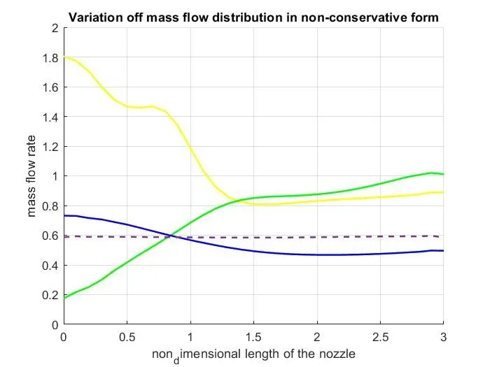
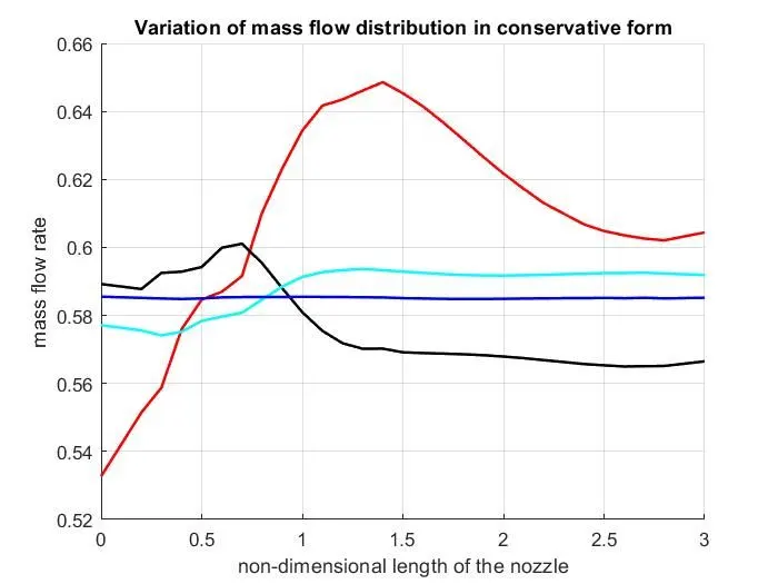
In the above two plots, Variation of mass flow distribution through nozzle at different times duting the time marching process for Non-conservative and conservative form of governing equations.

Let us compare the steady-state vatiations of mass flow obtained with the nonconservative and conservative forms of the governing equations (both after 1400 time steps-well beyond the time required to converge to the steady state). This comparision shows that the scale of the ordinate for mass flow is greatly magnified. Hence we see that the steady state mass flow distribution predicted by the conservation form of the equations is much more satisfactory than that obtained from the nonconservation form, which is because

• The conservation form gives a distribution that is much closer to being a constant. In contrast, the nonconservative results have 9on the magnified scale) a sizable variation, with some spurious oscillations at both inflow and outflow boundaries. Of course, on the practical basis, these variations are not apparent and mass flow essentially appears to be constant.

• The steady state mass flow results obtained with the conservative form are, on the whole, much closer to the exact analytical solution of p'A'V' = 0.579

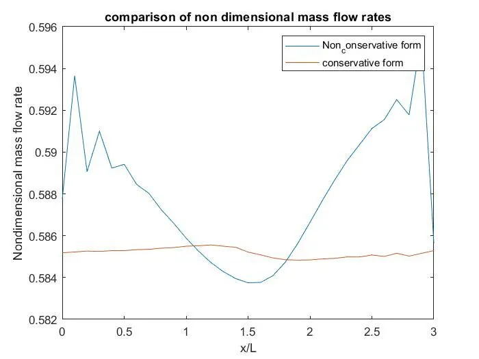
Figure shows a detailed comparison of the steady state mass flow variation(on a magnified scale) obtained with the nonconservative and conservative forms to the governing flow equation.

Solution for non conservative of steady state

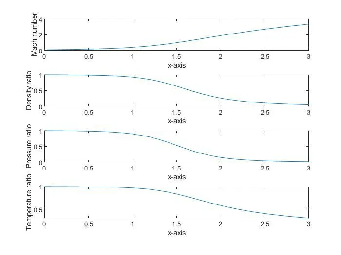
solution for consetrvative form at steady state

Grid Dependence test:

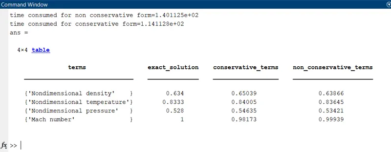
Note that the noncoservative form results are distinctly closer to the exact values. However, by doubling the number of grid points, the steady state numericals results in conservative form of governing equations are slightly closer to the exact analytical values (but still not as close as the nonconservative form with half as many grid points). For this projects, we have grid indepence with 31 grid points.

Results from the project

For the given flow problem, we cannot establish a clear superiority of the conservation form of the governing equations over the non-conservation from. However, we can make following observations:

1. The conservation form yeilds a better mass flow distribution. The conservation from simply does a better job of conserving mass.

2. The non-consevartive form leads to smallar residuals. The amount by which the computational time is slighly less, however it merely depends on the numerical algorithms in the first place.

3. There is no clear indication that which form yeilds better accuracy, though nonconservative form seems to produce slightly more accurate results for the primitive variables, and the conservative form seems to produce slightly more accurate results for flux variables. This results in either case are certainly satisfacotry.