Week 4 - CHT Analysis on Exhaust port
Aim : To carry out a Conjugate heat transfer analysis on an exhaust manifold.
Theory :
Conjugate heat transfer :
Conjugate heat transfer corresponds with the combination of heat transfer in solids and heat transfer in fluids. In solids, conduction often dominates whereas in fluids, convection usually dominates. Conjugate heat transfer is observed in many situations.
Why CHT analysis is used?
Conjugate heat transfer (CHT) analysis can accurately predict heat transfer by simultaneous solving all the relevant solid and flow field heat transfer processes, for example: conduction through solids, free and forced convection in the gases/fluids and thermal radiation.
The CHT approach has an advantage over FE Thermal analysis in that wall heat transfer coefficients and their local variations on surfaces are directly calculated within the model rather than based on simplified empirical calculations. The CHT approach therefore has benefits for those applications where heat transfer is either non-uniform or difficult to calculate empirically.
Where CHT analysis is used? (Application of CHT)
The heat is transferred from one fluid to the walls of the tube and then from the tube wall to other fluid. Here CHT analysis is useful for predicting the heat transfer coefficient and to improve the effective heat transfer rate. CHT is also used in analyzing the cooling of electronic devices.
Some Specific applications are: Cross Flow Heat Temperature, Integrated Circuit Chips, HVAC, Turbocharger, Internal Combustion Engine, Energy Saving applications etc.
Solving and modelling approach :
A. Geometry
1. Import the model in the spaceclaim.
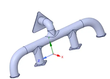
2. Remove the extra edges.
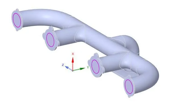
3. Extracting fluid volume by "Volume Extract" tool.
4. Sharing the topology by using "Share" tool which is available in workbench.
B. Meshing
1. Create following named selection
- Inlet
- Outlet
- Outer wall
- Inflation layer
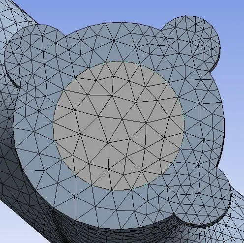
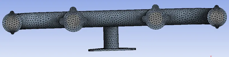
2. Create baseline mesh using default element size.
3. Mesh refinement
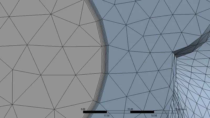
Insert inflation layer using appropriate thickness, based on the calculation of Y+ range for the particular turbulence model.
For K-Omega SST model ; Y+ = 1 to 5.
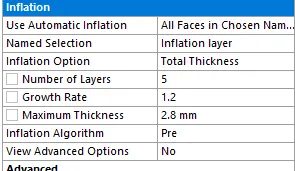
Inflation layer
C . Setup
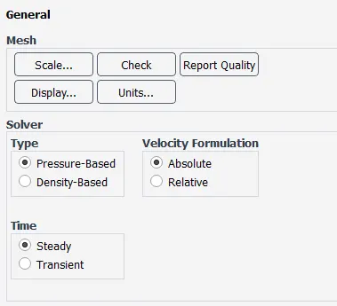
1. General
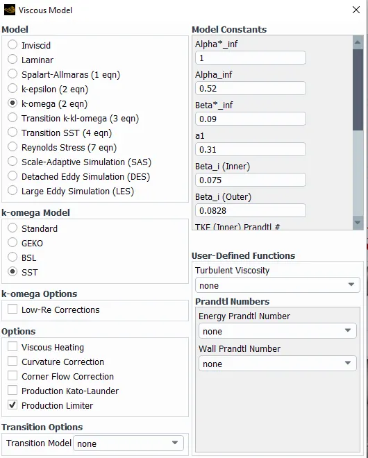
2. Turbulence model
K-omega SST model
3. Create material
For fluid material is air.
For solid material is aluminium.
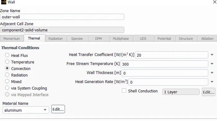
4. Create boundry conditions
Inlet : Velocity = 5 m/s , Temperature = 700K
Outer wall : HTC = 20 w/m2K , Temperature = 300 K
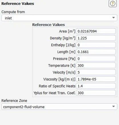
5. Reference values
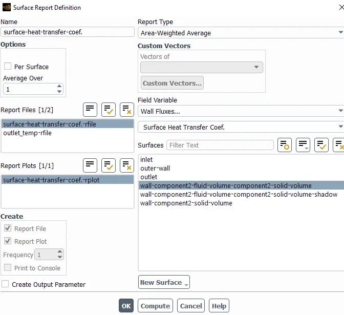
6. Create a report definition for the surface heat transfer coefficient.
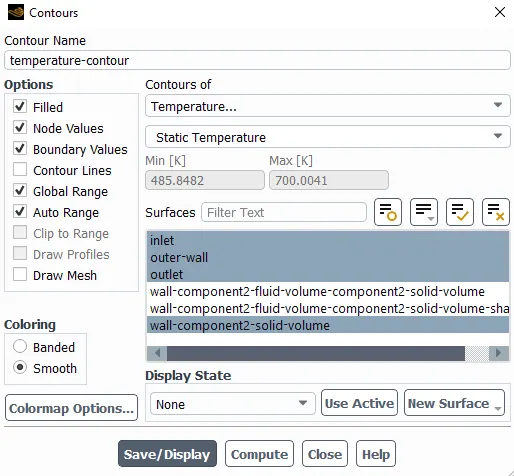
7. Create temperature contour
D. Post processing
Case 1 : Baseline Setup
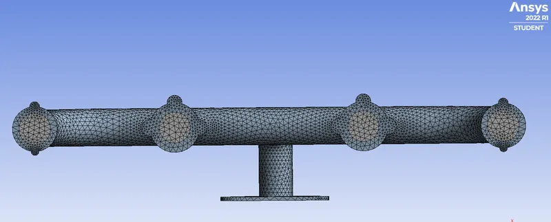
Meshing is done using default value of mesh size.
Meshing :

Results :
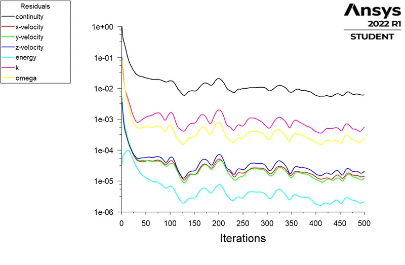
Residuals :
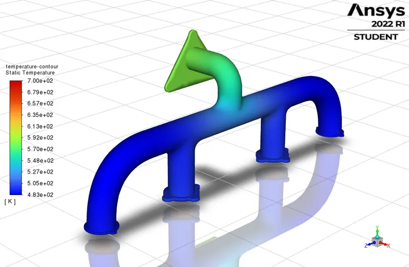
Temperature contour :
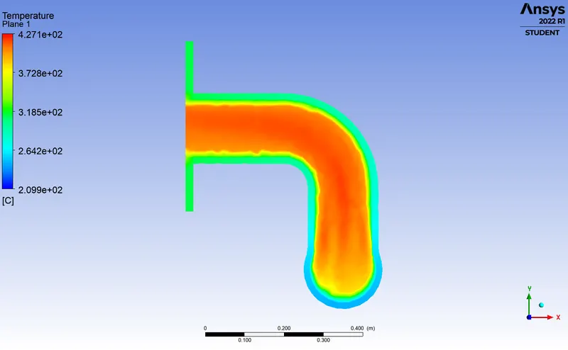
Temperature contour (cut plane) :
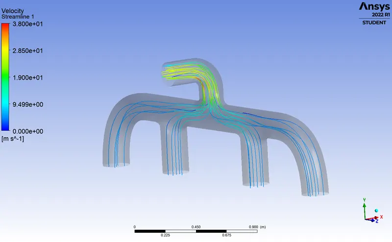
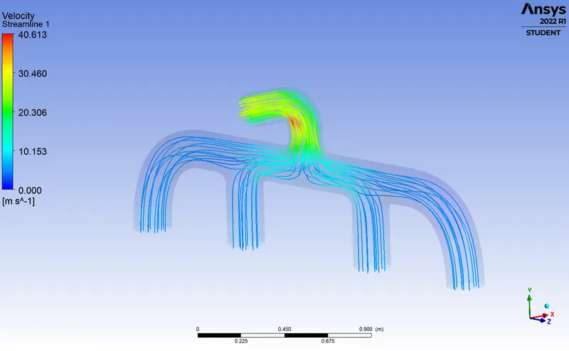
Velocity streamlines :
Velocity contour (cut plane) :
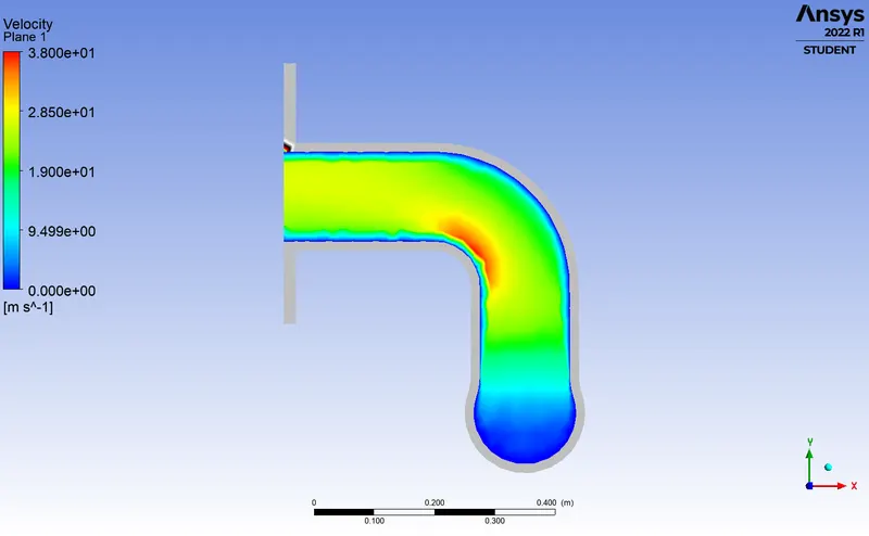
At the bend we can see the high velocity zone.
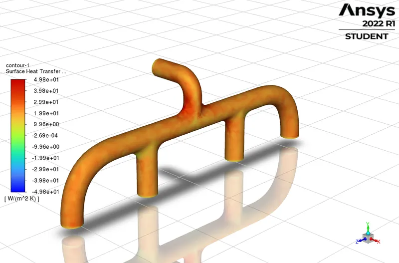
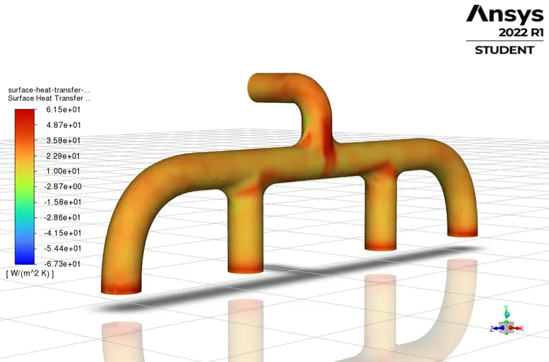
Surface heat transfer coefficient :
Case 2 : Refined Setup
Our area of intrest is to calculate the wall heat transfer coefficient we chose k-ω model as it is best for computing flow near the wall.
For K-omega SST model Y+ values are vary from 1 to 5 .
According to the Y+ first layer thickness is given to inflation layer in refined cases.
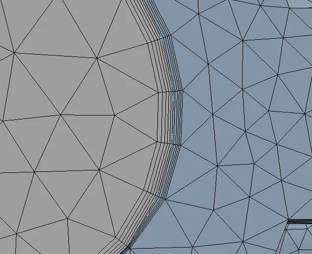
A) For Y+ =1 and Mesh size = 50 mm
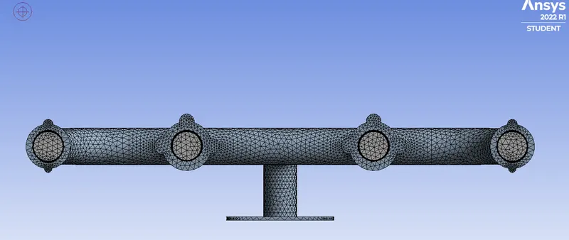
Meshing :

Results :
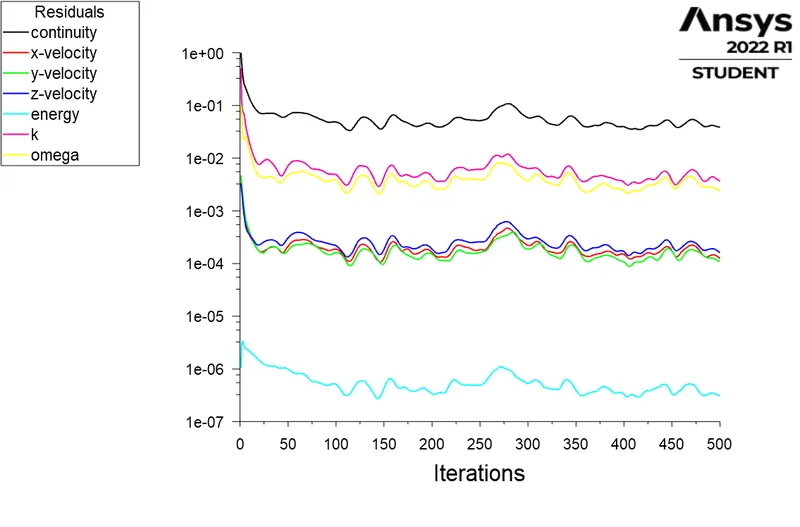
Residuals :
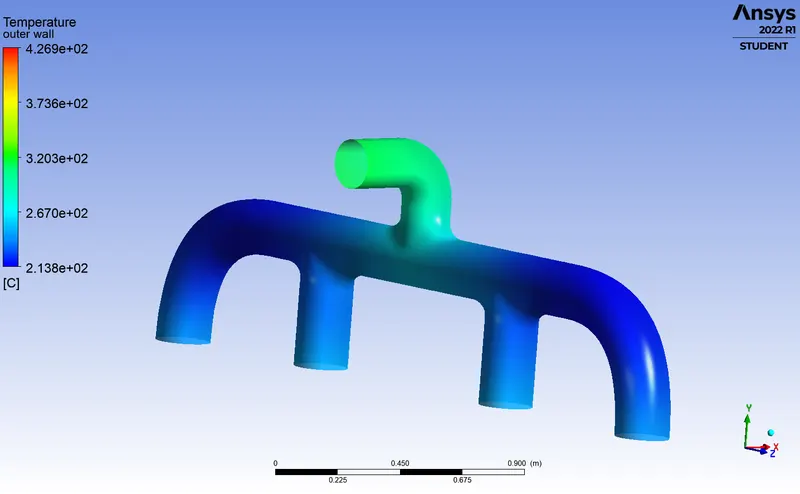
Temperature contour :
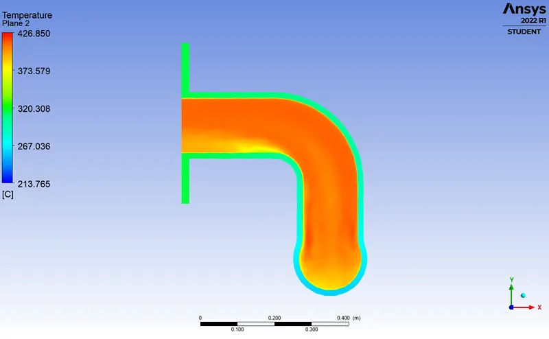
Temperature contour (cut plane) :
Velocity streamlines :
Velocity contour (cut plane) :
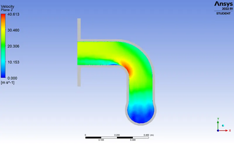
At the bend we can see the high velocity zone.
Surface heat transfer coefficient :
B) For Y+ =5 and Mesh size = 50 mm
Meshing :

Results :
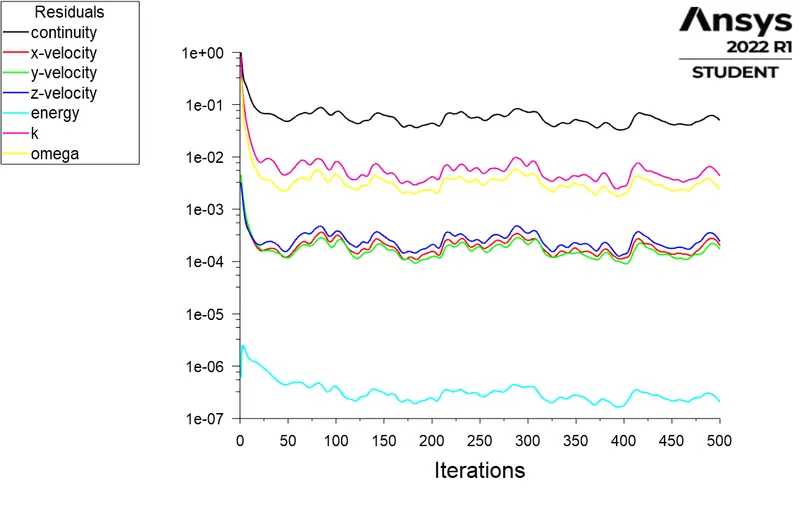
Residuals :
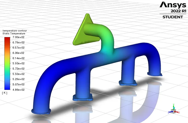
Temperature contour :
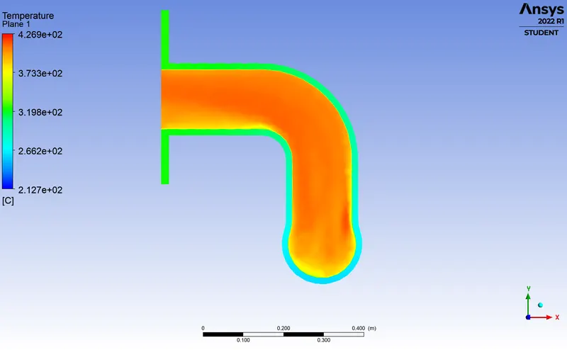
Temperature contour (cut plane) :
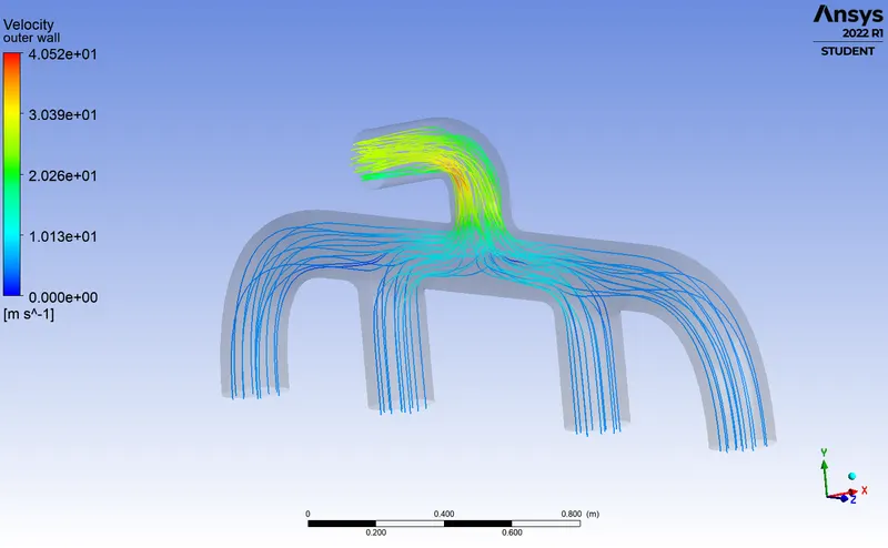
Velocity streamlines :
Velocity contour (cut plane) :
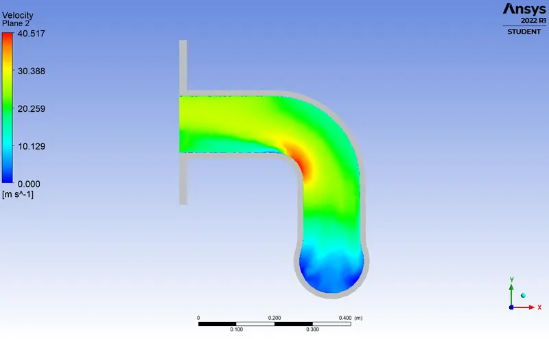
At the bend we can see the high velocity zone.
Surface heat transfer coefficient :
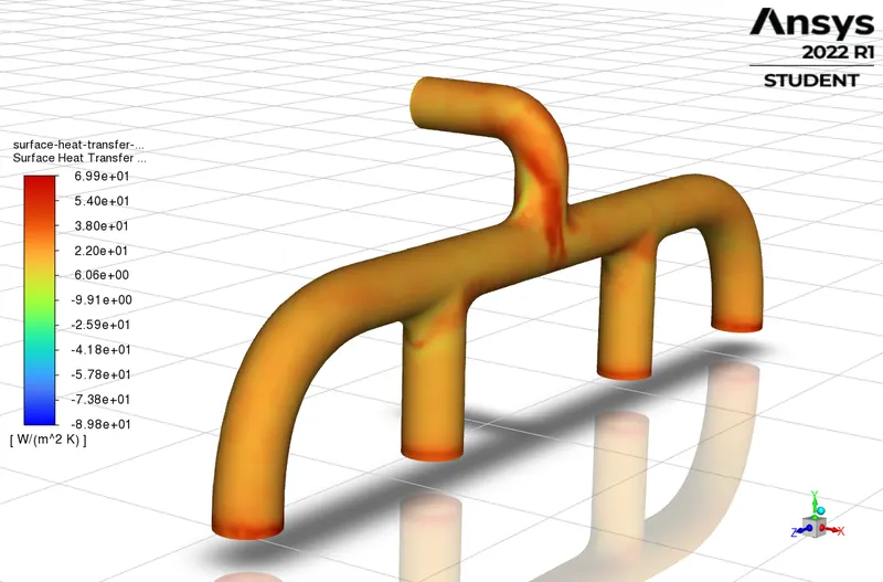
How would you verify if the HTC predictions from the simulations are right? On what factors does the accuracy of the prediction depend on?
Analytical method for calculating HTC :
`Nu=0.023*(Re^(0.8))*Pr^(n)`
Pr = Prandtl Number
Re = Reynold's number = `(rhoUL)/mu`
`Pr=v/alpha= (mu/rho)/(k/C_p)=(C_p*mu)/k`
Factors affecting the accuracy of prediction are as follows :
- Element Size and Quality - The finer the mesh, the accurate the results.
- Inflation Layer - It increases the quality of mesh near the boundary interface and helps to capture smooth plots of different quantities.
- Mesh at the solid-fluid interface - The mesh at the solid-fluid interface must be conformal.
Conclusions :
- With baseline meshing the wall adjacent HTC could not be computed. Thus inflation layer computes the wall adjacent HTC perfectly.
- The velocity at outlet is high due to the law of conservation of momentum
- Thus the velocity increases to a higher extent at outlet leading to high turbulence at the bends of the pipe.
- As we refine the mesh it take more time for computing.
- Since our area of intrest is to calculate the wall heat transfer coefficient we chose k-ω model as it is best for computing flow near the wall.
- Thus y+ assumed to be 1 and hence we calculate the first layer thickness of the inflation.