Week-4 Challenge WOT Condition Part-2
1. What is the difference between mapped and dynamic model of engine, motor and generator? How can you change model type?
Ans: -
Mapped Model
- Model uses a set of steady-state lookup tables to characterize engine performance.
- Mapped models are used when the behavior of a particular model is not of our interest and can be modeled with predefined values in the form of lookup tables.
- Mapped model is going to work faster and it runs based on the data given in the lookup table.
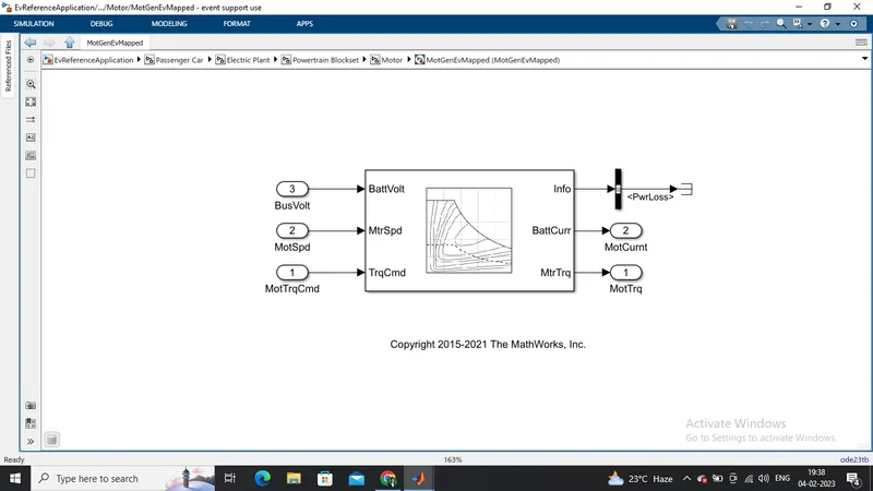
- Implements a mapped motor and drive electronics operating in torque control mode. we have to specify electrical torque range with a torque-speed envelope or maximum motor power and torque.
- Output torque tracks a torque reference demand and includes a motor and drive response time constant.
- Also have to Specify electrical losses as a single operating point that estimates loss across the operating range, measured loss, or measured efficiency.
Dynamic Model
-
Dynamic model is used if you need a more detailed dynamic model and have component-level data.
-
Dynamic model is used to analyze the impact of individual engine components on the overall performance & it is going to represent actua components.
- Dynamic models are used when the internal response to a model with respect to its components is needed.
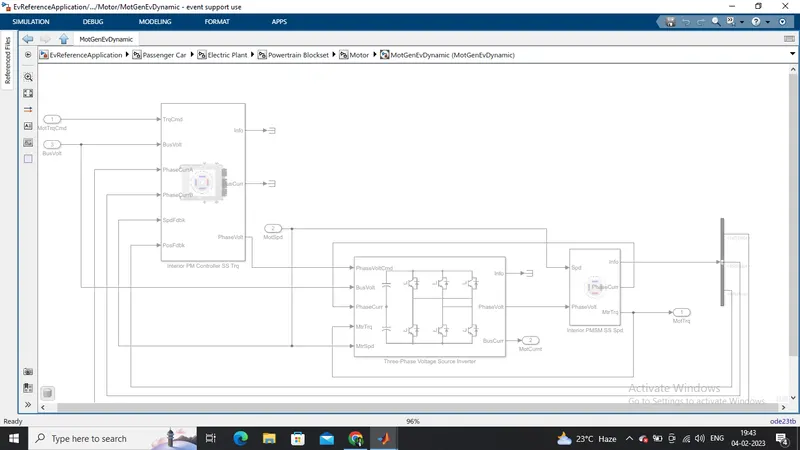
Changing the model type in EV powertrain blocks
- we can use the variant manager in the modeling tab to find the variant systems we have. Right-click on the model you want and use set as Label mode active choice.

2.How does the model calculate miles per gallon? Which factors are considered to model fuel flow?
Ans: -
Below is the highlighted simulink block to calculate miles per gallon.
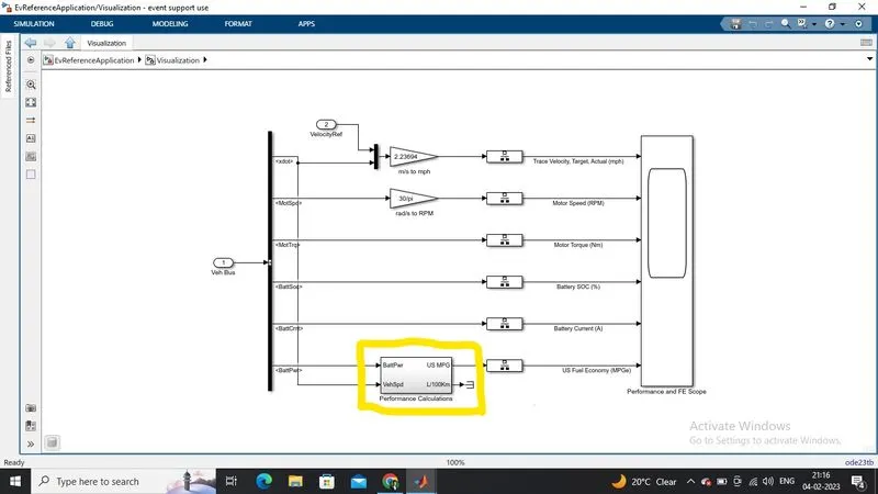
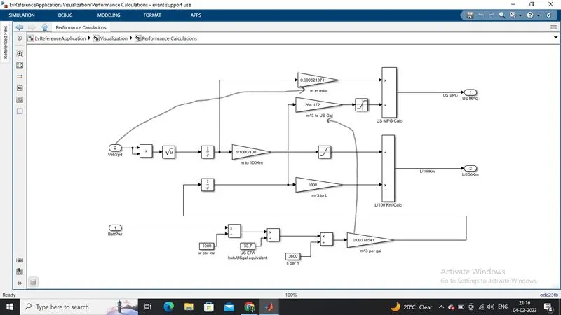
- Vehicle speed data is used to calculate the distance traveled in meters which is then converted to miles
- Battery power data is used to find power used in kWh which is then converted to gasoline-equivalent using US EPA value by dividing with 33.7
- Note: As per the US environmental protection agency(EPA) 1 gallon of gasoline is equal to 33.7 kWh
- Dividing distance traveled in miles by the number of gallons, we can get miles per gallon.
- For HEV this gallon(gasoline-equivalent of battery power) is added with gallon used by IC engine then miles per gallon is calculated.
3. Run the HEV ReferenceApplication with WOT drive cycle. Change the grade and wind velocity in the environment block. Comment on the results.
Ans: -
Simulation of HEV with WOT condition without any change
The simulink window of the HEV reference application and the modified drive cycle source window is show below.
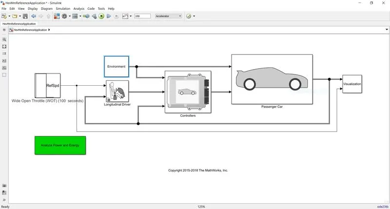
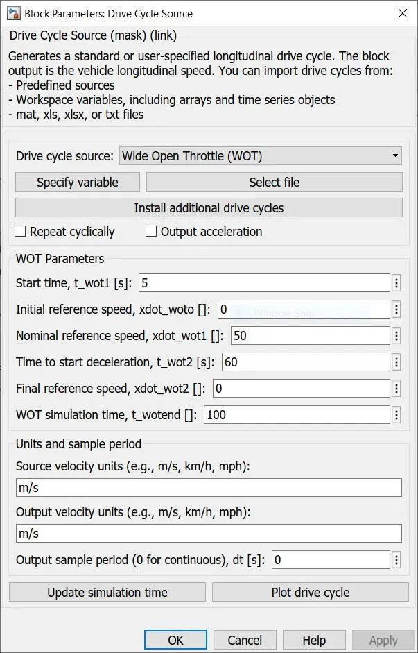
The drive cycle source is modified in such a manner to simulate the vehicle in wide open throttle condition.
The result of the simulation
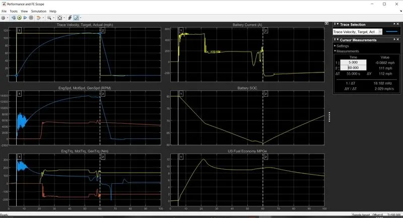
The result consists of six plots in which ,
Plot 1 - Target speed vs Actual speed in mph
The top speed of 112 mph was achieved in 42.3 seconds
The deceleration from 112 mph - 0 mph was achieved in 7.5 seconds
Plot 2 - Speed curve of engine , motor speed and generator speed
This shows the speed of the engine, motor and generator at various points
Plot 3 - Torque curve of engine, motor and generator in N-m
The torque of generator is in negative @ 21 sec of the simulation, which shows that the battery is getting recharged.
The torque of engine is reduced gradually as the power increases, due to the speed requirement of the vehicle.
Plot 4 - Battery current
Initially the current required to run the motor is high and reduces when the speed of the vehicle increases. The motor is used mainly for the starting torque of the vehicle since, the current requirement of the motor is also high.
Plot 5 - Battery state of charge
Initially the state of charge is at 80%. At the end of acceleration the SOC becomes 60.06%. This change in SOC shows the use of motor while acceleration. At 21 sec of the simulation the generator starts recharging the battery. Therefore two different discharging slopes occur during the acceleration of the vehicle.
When the vehicle starts decelerating, the state of charge gradually increases as there is no usage of motor and the generator continues to recharge the battery.
Plot 6 - Fuel economy
The fuel economy in US MPG which is calculated in the performance calculation block of the model is shown in this plot.
The fuel economy was high until the motor was used to accelerate the vehicle. When the power requirement of the vehicle increases the fuel economy decreases respectively
The maximum fuel economy was 12.04 MPG
The minimum fuel economy obtained was 7.18 MPG
Simulation of HEV with WOT condition with changes in environment block
The parameters of the drive cycle source block is kept the same.
The parameters such as grade and wind velocity in the environment block is changed as shown below
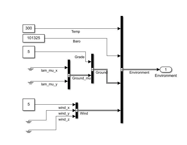
>The Grade value is set to 5 degrees
>The wind velocity is set to 5 m/s in x axis direction
>Other parameters remains unchanged
The result of simulation
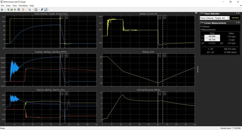
The result consists of six plots in which ,
Plot 1 - Target speed vs Actual speed in mph
The top speed of 85.1 mph was achieved in 55 seconds
The deceleration from 85.1 mph - 0 mph was achieved in 5.31 seconds
Plot 2 - Speed curve of engine , motor speed and generator speed
This shows the speed of the engine, motor and generator at various points
Plot 3 - Torque curve of engine, motor and generator in N-m
The torque of generator is in negative @ 21 sec, which shows that the battery is getting recharged.
The torque of engine is reduced gradually as the power increases, due to the speed requirement of the vehicle.
Plot 4 - Battery current
Initially the current required to run the motor is high and reduces when the speed of the vehicle increases. The motor is used mainly for the starting torque of the vehicle since, the current requirement of the motor is also high.
Plot 5 - Battery state of charge
Initially the state of charge is at 80%. At the end of acceleration the SOC becomes 60.03%. This change in SOC shows the use of motor while acceleration. At 21 sec of the simulation the generator starts recharging the battery. Therefore two different discharging slopes occur during the acceleration of the vehicle.
When the vehicle starts decelerating, the state of charge gradually increases as there is no usage of motor and the generator continues to recharge the battery.
Plot 6 - Fuel economy
The fuel economy in US MPG which is calculated in the performance calculation block of the model is shown in this plot.
The fuel economy was high until the motor was used to accelerate the vehicle. When the power requirement of the vehicle increases the fuel economy decreases respectively
The maximum fuel economy was 9.17 MPG
The minimum fuel economy obtained was 5.11 MPG
Conclusion
The results are compared using a spreadsheet
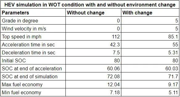
Hence we can conclude that the vehicle with lower degree grade and lower wind velocity,
>Can reach high speed in short amount of time.
>Have high fuel efficiency.
>Have high deceleration time.
>Have better SOC.
Simulation of pure electric vehicle with WOT drive cycle
Simulation of Pure EV with WOT condition without any change
The drive cycle source window parameters are kept similar to the HEV simulation.
The simulation is made to run with no change in the environment block.
The result of the simulation
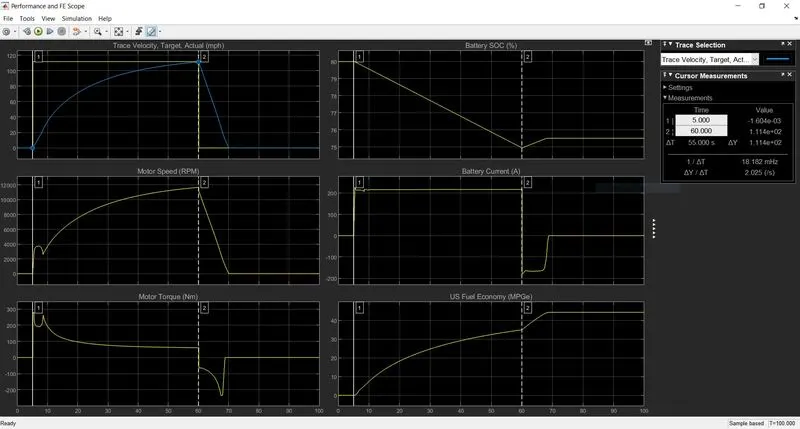
The result consists of six plots in which ,
Plot 1 - Target speed vs Actual speed in mph
The top speed of 111.4 mph was achieved in 55 seconds
The deceleration from 111.4 mph - 0 mph was achieved in 10 seconds
Plot 2 - Speed curve of motor
This shows the speed of the motor at various points in rpm
Maximum motor speed - 11670 rpm
Plot 3 - Torque curve of motor in N-m
The torque of motor is in negative from 60 sec - 70 sec, which shows that the vehicle is decelerating and the battery is getting recharged
Plot 4 - Battery current
The battery current requirement in the WOT condition for the vehicle was constant until the acceleration of the vehicle stops.
During deceleration, the current value goes negative which shows that the battery is recharged during that period of time.
Plot 5 - Battery state of charge
Initially the state of charge is at 80%. At the end of acceleration the SOC becomes 74.94%. This change in SOC shows the use of motor while acceleration. During the 10 sec deceleration period, from 60 sec - 70 sec of the simulation the battery got charged by 0.56%. therefore the SOC at the end of simulation was 75.50%
Plot 6 - Fuel economy
The fuel economy in US MPG which is calculated in the performance calculation block of the model is shown in the plot.
The maximum fuel economy was 44.30 MPG
The minimum fuel economy obtained was 34.95 MPG
Simulation of Pure EV with WOT condition with changes in environment block
>The drive cycle source window parameters are kept similar to the HEV simulation.
>The Grade value is set to 5 degrees
>The wind velocity is set to 5 m/s in x axis direction
>Other parameters remains unchanged
The simulation is made to run with the above changes
The result of the simulation
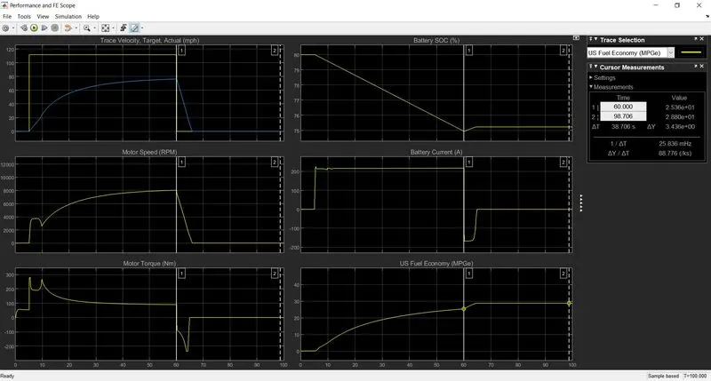
The result consists of six plots in which ,
Plot 1 - Target speed vs Actual speed in mph
The top speed of 76.36 mph was achieved in 55 seconds
The deceleration from 76.36 mph - 0 mph was achieved in 6 seconds
Plot 2 - Speed curve of motor
This shows the speed of the motor at various points in rpm
Maximum motor speed - 8046 rpm
Plot 3 - Torque curve of motor in N-m
The torque of motor is in negative from 60 sec - 66 sec, which shows that the vehicle is decelerating and the battery is getting recharged
Plot 4 - Battery current
The battery current requirement in the WOT condition for the vehicle was constant until the acceleration of the vehicle stops.
During deceleration, the current value goes negative which shows that the battery is recharged during that period of time.
Plot 5 - Battery state of charge
Initially the state of charge is at 80%. At the end of acceleration the SOC becomes 74.94%. This change in SOC shows the use of motor while acceleration. During the 6 sec deceleration period, from 60 sec - 66 sec of the simulation the battery got charged by 0.23%. therefore the SOC at the end of simulation was 75.23%
Plot 6 - Fuel economy
The fuel economy in US MPG which is calculated in the performance calculation block of the model is shown in the plot.
The maximum fuel economy was 28.8 MPG
The minimum fuel economy obtained was 25.36 MPG
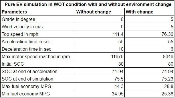
>Can reach high speed in short amount of time.
>Have high fuel efficiency.
>Have high deceleration time.
>Due to high deceleration time, the recharging time of battery is also high
>Therefore better SOC
Comparing the conclusions of simulations of HEV and Pure EV
A spreadsheet is used to compare the results of all the four simulation as shown below
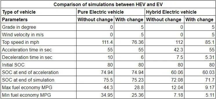
It is clearly seen that,
>HEV and EV without changed parameters have approximately equal top speeds. Since there is no opposing environmental forces
>HEV has good acceleration time. Since it has both motor and a engine.
>HEV with changed environment parameters has the lowest deceleration time.
>Pure EV with unchanged environment parameters has the longest deceleration time.
>Initial SOC of all the vehicles are same.
>At the end of acceleration EV has better SOC compared to the HEV simulation.
>SOC at the end of all the simulations is approximately equal.
>Pure EV without changed parameters has high fuel economy when compared to other simulations.
>HEV with changed parameters has the lowest fuel economy.