Week-4 Challenge WOT Condition Part-2

1. What is the difference between mapped and dynamic model of engine, motor and generator? How can you change model type?

A:

• Powertrain blockset in MATLAB consists of two models: Mapped and dynamic model.
• Dynamic model represents actual model and components. Static model works faster and runs based on the data in the lookup table.
• Mapped engine block implements a mapped spark ignition model using power, air mass flow, fuel flow, exhaust temperature, efficiency and emission performance lookup tables.
• Dynamic model decomposes the engine behavior into engine characteristics that are seperated into lower level components. By combining components in this way the model captures the dynamic effects.
• Mapped models are used for quasi steady state engine simulations.
• Dynamic model is used to analyse the impact of individual engine components on the overall performance.

EV reference model:

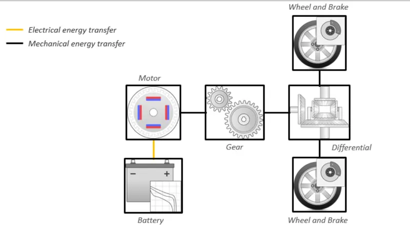
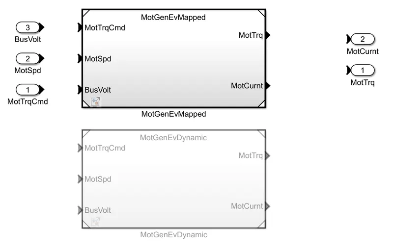
The figure below shows the mapped engine and the dynamic engine part is not connected (command out):

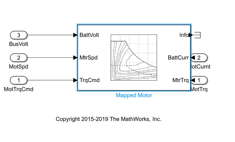
Dynamic engine model simulation blocks:

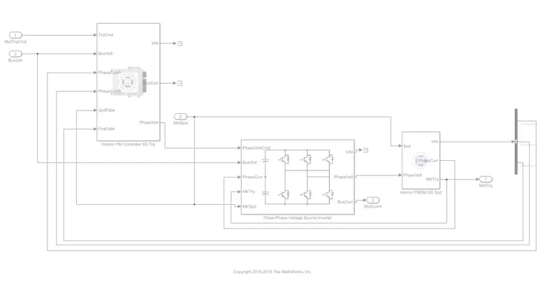
To switch between mapped and dynamic engine :

• Open the EV model file from the powertrain blockset in the help option.
• The model will be opening in Simulink window.
• Inside the passenger car block click on the EV Motor/Generator block.
• Then right click on it and select variant label with options MotGenEvDynamic or MotGenEvMapped.
• Finally select the Label mode active choice.

2. How does the model calculate miles per gallon? Which factors are considered to model fuel flow?

A:

• Miles per gallon is a fuel efficiency calculation method in conventional gasoline vehicles. But in case of HEVs the fuel efficiency is calculated using Miles per gallon equivalent.
• Miles per gallon is the number of miles the car can travel per gallon of gas.
• Miles per gallon equivalent rate is calculated by finding the number of miles the vehicle can go using the same energy content as gallon of gas.
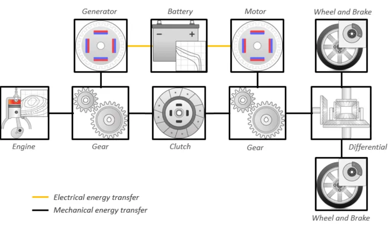
• Hev Multimode Reference application schematic:

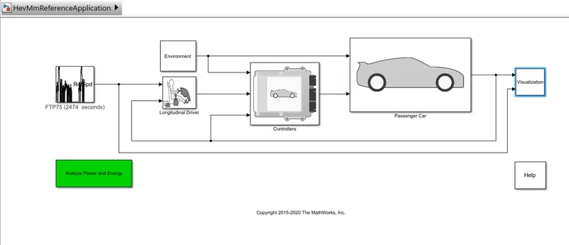
• HevMm reference application simulation model:

• Inside the visualization block click on perfrmance calculation block.

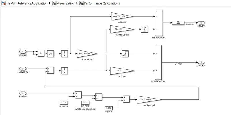
• Here in the above performance calculation block miles per gallon is obtained from calculating 3 inputs.
• The inputs provided are : Vehicle speed , Fuel flow , Battery power.
• Vehicle speed is integrated to find the distance with respect to time. It is then converted to miles by mutiplying with 0.000621371.
• Fuel flow is expressed as mass flow rate (kg/sec) and it integrated to convert mass of fuel to volume and then multiply with 1000 to convert in to litres and then to US gallon by multiplying with 264.172
• Battery power value is first converted to kwh by dividing the watts with 1000 and converted to gallon by dividing it with 33.7 as shown in the figure. Then it is divided with 3600 to convert to per seconds and then finally multiply with 0.00378541 to convert into cubic meter per gallon.
• All these converted inputs from vehicle speed and fuel flow (equivalent gallon) is further divided and result is obtained in Miles/Gallon.

3. Run the HEV ReferenceApplication with WOT drive cycle. Change the grade and wind velocity in the environment block. Comment on the results.

A:

• HEV architecture uses more than i source for propulsion power. If hybrid is done through the battery or electric technology then it is HEV.
• The figure below shows Hev Multimode Reference Application model taken from power train blockset.

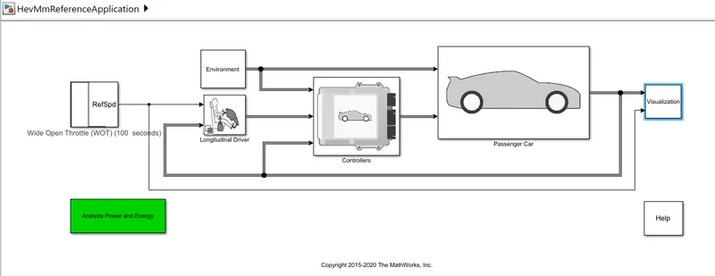
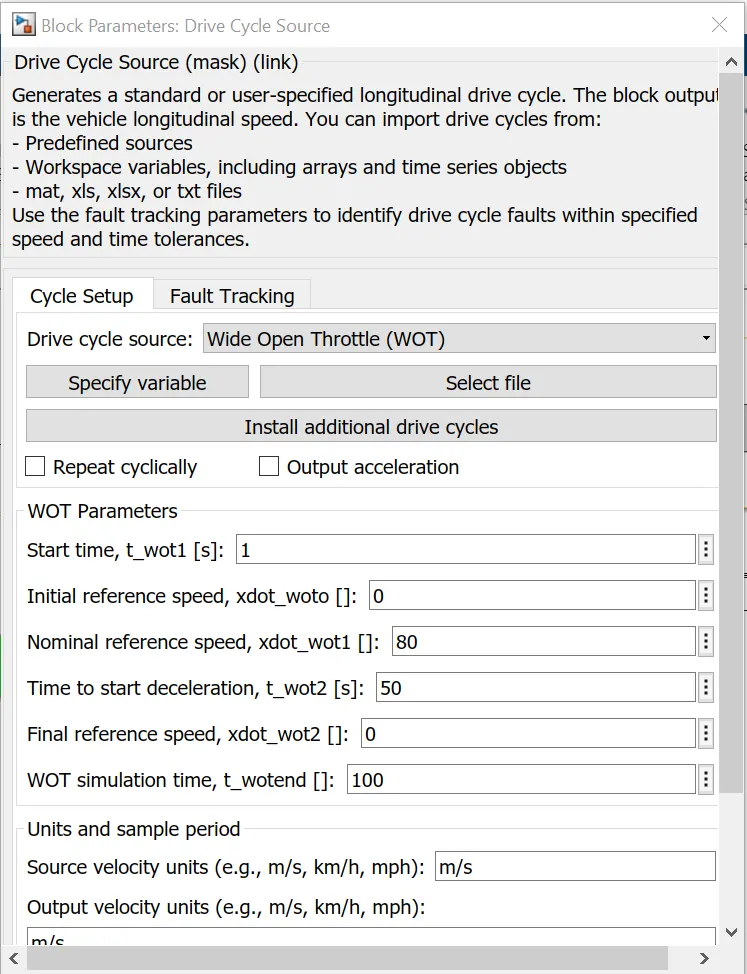
• Drive cycle input is changed to Wide Open Throttle and the cycle setup readings or the input parameters are selected as random values as per the image shown below.

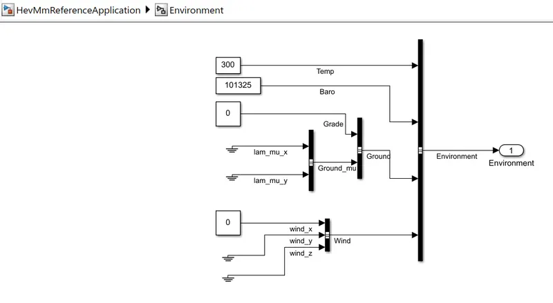
• Inside the Environment block there is grade and wind velocity parameters.
• Initially the grade and wind velocity value is kept as zero.

• Simulation output with 6 plots:

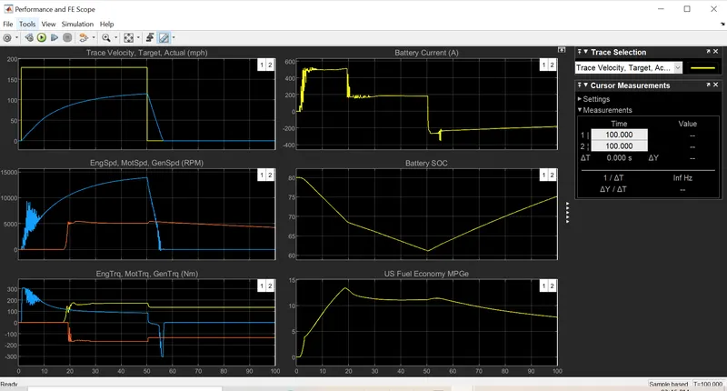
• Here in the plot obtained there is a curser measurement which helps us to study about the measurements or values or nature of graph with respect to time according to acceleration of vehicle.
• Plot 1: Shows velocity versus time with respect to the drive cycle data provided. Acceleration time required to reach 80 mph is 16.7 seconds. Deceleration time required to reach minimum from 80 mph is 6.2 seconds.
• Plot 2: Shows the changes in speed of engine, motor and generator in rpm throughout the drive cycle. Peak engine speed = 4780 rpm, peak motor speed = 9497 rpm, peak generator speed = 13690 rpm.
• Plot 3: Shows torque characteristics and changes in engine, motor and generator throughout the drive cycle. Peak engine torque = 138.7 Nm, Peak motor torque = 206.7 Nm, Peak generator torque = 42.2 Nm.
• Plot 4: Shows the battery current values and its changes for various acceleration inputs. The peak current discharge from the battery = 163.5A, Peak current charging to the battery = -150.86A
• Plot 5: Shows the battery state of charge and its changes. The SOC decreased from 60% to 39.8% of charge in time period of 49.3 seconds.
• Plot 6: Shows the fuel economy as miles per gallon for the given driving cycles. Maximum miles the vehicle can run per gallon of fuel equivalent = 46 miles.

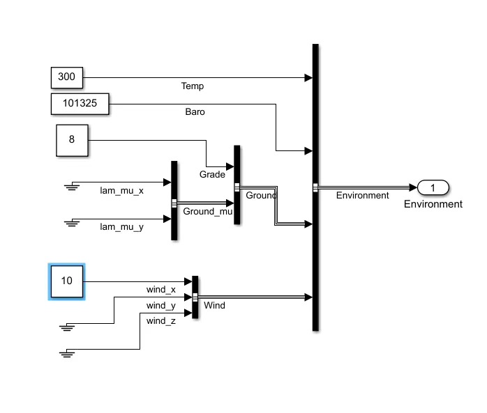
CASE 2: WOT drive cycle inputs are kept same. Grade angle is changed from 0 to 8 degrees.

Wind velocity is changed from 0 to 10 m/s. we can take any values randomly.

• Simulation output with 6 plots:
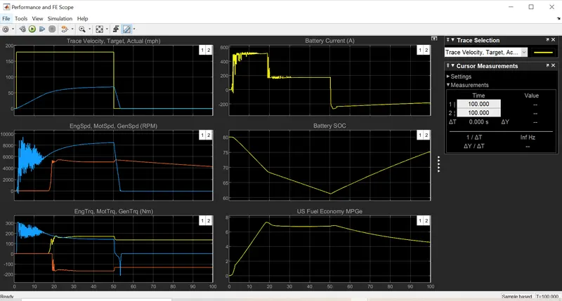
• Plot 1: Top speed of 80 mph cannot be achieved because of the additional forces acting and the vehicle runs upto 67.2mph. Acceleration time to reach top speed of 67.2 mph = 44.5 sec. Deceleration time from 80 to minimum= 5.06 sec.
• Plot 2: Peak engine speed = 4676 rpm, Peak motor speed = 8103.5 rpm, Peak generator speed = 12858.5 rpm.
• Plot 3: Peak engine torque= 139.6 Nm, Motor torque= 206.4 Nm, Peak generator torque= 48.2 Nm.
• Plot 4: Peak current discharge from battery =167.6A, Peak current charging to battery = -152.46A.
• Plot 5: SOC decreased from 60% to 25.98% of charge in timeperiod of 49.3 sec.
• Plot 6: Max miles the car can run per gallon of fuel equivalent= 17.93 Miles.

4. Keeping all other parameters same, compare the simulated results of hybrid and pure electric powertrains.

A:

• A pure EV or EV reference application model from powertrain blockset is selected.

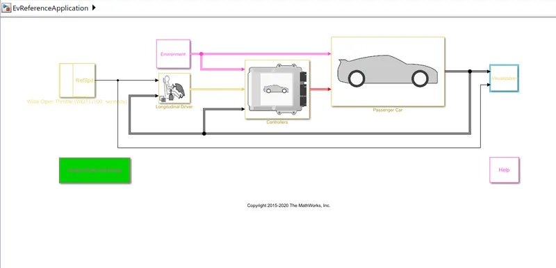
• Drive cycle is selected to be WOT and simulation parameters are varied as shown in the figure below.

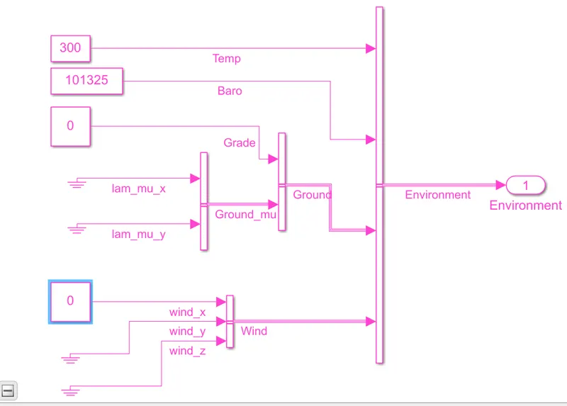
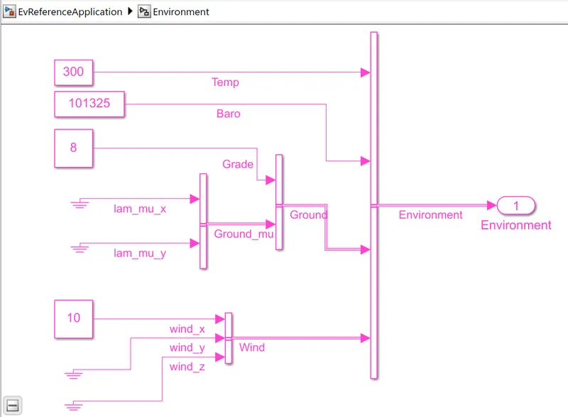
• Inside the Environment block there is grade and wind velocity parameters.
• Initially the grade and wind velocity value is kept as zero.

• Simulation output with 6 plots:

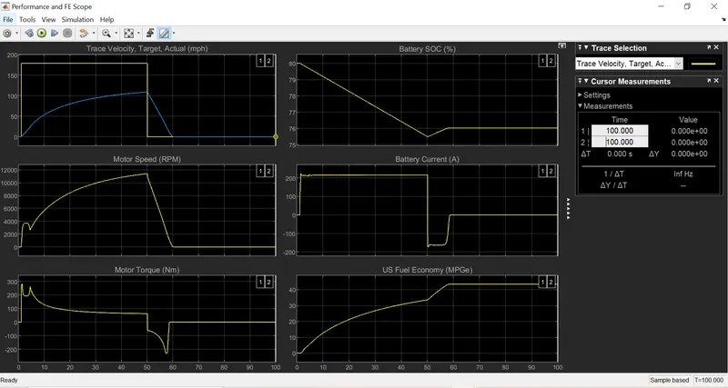
• Here in the plot obtained there is a curser measurement which helps us to study about the measurements or values or nature of graph with respect to time according to acceleration of vehicle.
• Plot 1: Shows velocity versus time with respect to the drive cycle data provided. Acceleration time required to reach 108.9 mph is 50.2seconds. Deceleration time required to reach minimum from 80 mph is 9.8 seconds.
• Plot 2: Shows the changes in speed of engine, motor and generator in rpm throughout the drive cycle. Peak motor speed = 11230 rpm.
• Plot 3: Shows torque characteristics and changes in engine, motor and generator throughout the drive cycle. Peak motor torque = 260Nm.
• Plot 4: Shows the battery current values and its changes for various acceleration inputs. The peak current discharge from the battery = 216.8A, Peak current charging to the battery = -173.7A
• Plot 5: Shows the battery state of charge and its changes. The SOC decreased from 80% to 75.5% of charge in time period of 50.3 seconds.
• Plot 6: Shows the fuel economy as miles per gallon for the given driving cycles. Maximum miles the vehicle can run per gallon of fuel equivalent = 20.45 miles.

CASE 2: WOT drive cycle inputs are kept same. Grade angle is changed from 0 to 8 degrees.

Wind velocity is changed from 0 to 10 m/s. we can take any values randomly.

• Simulation output with 6 plots:

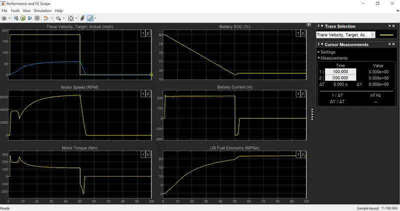
• Plot 1: Top speed of 80 mph cannot be achieved because of the additional forces acting and the vehicle runs upto 58.9mph. Acceleration time to reach top speed of 58.9 mph = 48.8 sec.
• Plot 2: Peak motor speed = 6254 rpm
• Plot 3: Peak Motor torque= 280 Nm
• Plot 4: Peak current discharge from battery =225.8A, Peak current charging to battery = -163.7A.
• Plot 5: SOC decreased from 80% to 75.5% of charge in timeperiod of 49 sec.
• Plot 6: Max miles the car can run per gallon of fuel equivalent= 21.45 Miles.

Comparison (HEV and Pure EV):

Here both ev and hev are simulated under same environmnental and drive cycle condition:

• EV results in less top speed achievement compared to HEV.
• SOC improvement of 15% is seen in HEV during deceleration and only 1% in EV.
• Peak motor speed is less in EV compared to HEV.
• During deceleration negetive current flows more time in HEV than EV.
• Emmissions are more in HEV than EV.