Week-4 Challenge WOT Condition Part-2

Week-4 Challenge WOT Condition Part-2

AIM:

1. What is the difference between mapped and dynamic model of engine, motor and generator? How can you change model type?
2. How does the model calculate miles per gallon? Which factors are considered to model fuel flow?
3. Run the HEV Reference Application with WOT drive cycle. Change the grade and wind velocity in the environment block. Comment on the results.
4. Keeping all other parameters same, compare the simulated results of hybrid and pure electric powertrains.

SOLUTION:

Mapped Model:

Mapped model is a model used where the model is designed not in practical cases, but modeled by entering the interested values in the lookup table for obtaining the Simulink result.

Dynamic Model:

Dynamic model used when the actual result of the component is required and not with the interested values.

Engine

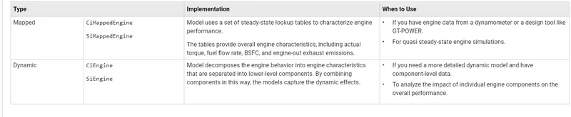
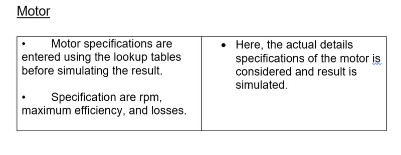
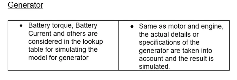
Changing from Mapped to dynamic model:

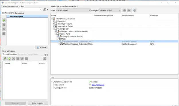
If model needs to be changed from mapped to dynamic, click the Variant Manager and select the Dynamic option. Right click on the Dynamic motor and select the Set as label Mode Active Choice.

2.

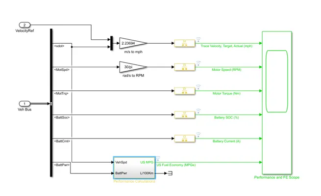
Open the EV reference application model in MATLAB. Now open the visualization block where the parameters used for calculating miles per gallon are given.

Then open the performance calculation block.

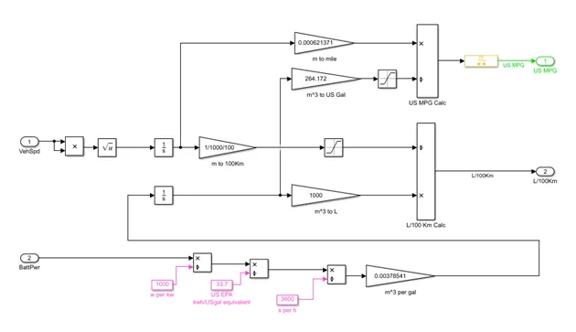
The input given for calculating miles per gallon are Vehicle speed, Battery power and Fuel flow.

We know that 1 US liquid gallon equal to 3.78 litres. i.e. 264.17 gallon equals 1000 litres. The vehicle speed is multiplied with itself and square rooted. The value is then integrated and converted to meters. Then meter to miles and its is divided by US gal . For US gal we need to divide battery power by 1000 and then divide again by 33.7. Now it is converted from sec to hr by dividing with 3600 to convert to m^3 per gal. The final value is converted to gal and used as MPG.

3.

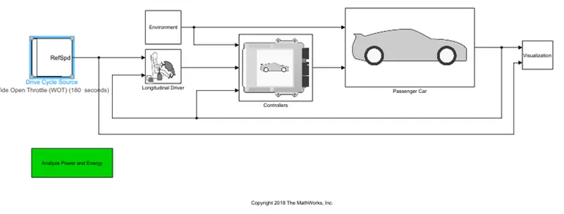
Now change the drive cycle to wide open throttle.

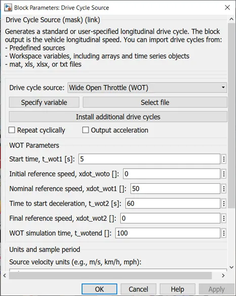
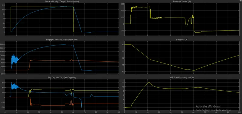
For Grade =0 and wind velocity=0,

For Grade=5 and wind velocity=10,

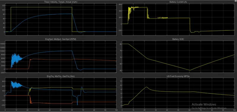
Plot 1: Shows the analysis between Target velocity Vs Actual velocity.

Plot 2: Provides the analysis between Engine speed and Motor Speed.

Plot 3: Shows comparison between Engine torque, motor torque and generator torque.

Plot 4: Power produced by battery.

Plot 5: Battery’s State of Charge.

Plot 6: Fuel efficiency denoted in Miles per Gallon.

By comparing the Two graph plots, increase in grade and wind velocity, results in

• Peak velocity reduces as gradient and aerodynamic forces becomes dominant.
• Fuel economy also reduces as distance travelled reduces.
• Deceleration time reduces so that regeneration capacity also affects.

4.

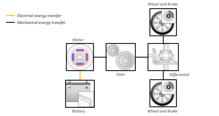
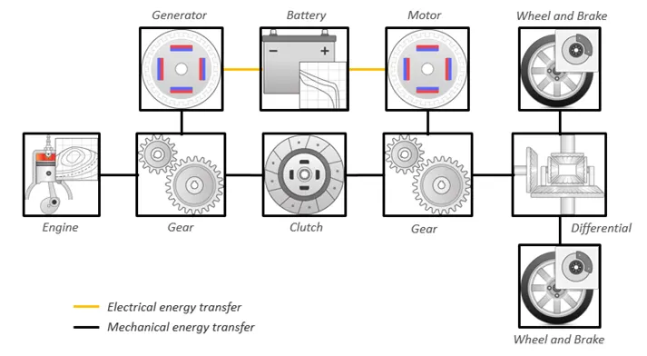
Comparing the simulated results of hybrid and pure electric powertrains with same parameters.

Model Configurations:

EV:

HEV:

Simulink Model:

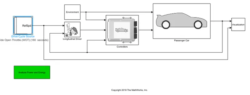
By Keeping the Grade and Wind velocity common for both the EV and HEV models, below graphs are plotted.

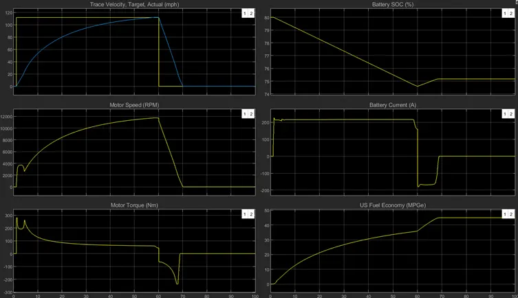
EV:

HEV:

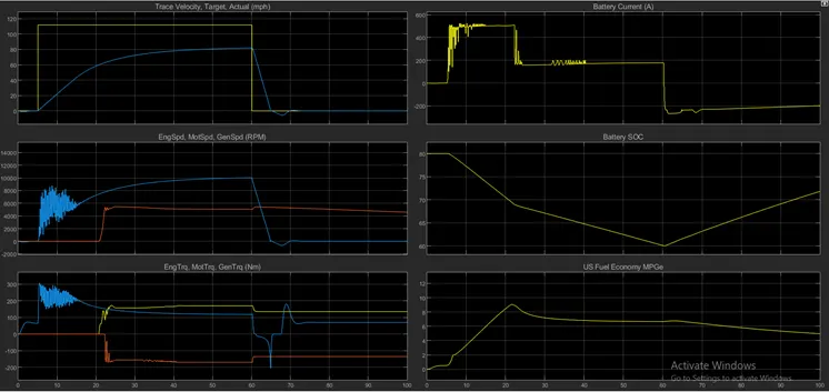
Conclusions from the above plots are

• Pure Electric Vehicle have low velocity compared to Hybrid Electric Vehicle.
• Deceleration time is low for HEV compared to EV.
• Motor speed is also less than HEV, but path tracings is same as that of HEV.
• Motor Torque of EV is almost Similar to HEV.
• Fuel Economy is more for EV compared to that HEV Due to more number of moving parts in HEV Compared to EV