Introduction to HEV using MATLAB and SIMULINK: Wide - Open Throttle [Case 2] (#04)
AIM:
The aim of this challenge is to understand the basics of the Powertrain Blocksets offered by Mathworks as extension to SimuLink.
OBJECTIVES:
1. To understand the difference between mapped and dynamic model of engine, motor and generator.
2. To understand the theory behind calculating miles per gallon using Powertrain Blockset models and to identify the factors that are important to model fuel flow.
3. To simulate the HEV Reference Application with WOT drive cycle and analysing results after changing the grade and wind velocity in the environment block.
4. To simulate and compare the simulated results of hybrid and pure electric powertrains.
Powertrain Blockset:
Powertrain Blockset™ provides fully assembled reference application models of automotive powertrains, including gasoline, diesel, hybrid, and electric systems. It includes a component library for simulating engine subsystems, transmission assemblies, traction motors, battery packs, and controller models. Powertrain Blockset also includes a dynamometer model for virtual testing.
Powertrain Blockset provides a standard model architecture that can be reused throughout the development process. You can customize models by parameterizing components in a reference application with your own data or by replacing a subsystem with your own model.
Cool things one can do with Powertrain Blockset:
a) Engine control design / calibration
b) Design optimization studies
c) Multidomain simulation via SimScape
d) Subsystem control design
e) Hardware-in the loop (HIL) testing
f) Design trade-off analysis for automotive systems.
STUDY 1:
To understand the difference between mapped and dynamic models of engine, motor and generator.
There are two types of models for various subsystems like engine, motor, generator etc:
| Mapped Models | Dynamic Models | |
| Definition | Mapped models represent the macro behavior of the subsystem as a set of lookup tables. These models are useful for understanding the behaviour of the subsystem using empirical data. | Dynamic models decompose the subsystem behavior into individual component models. |
| Uses | Mapped models are suitable for analysis and design activities that do not require subsystem dynamic characteristics, for example, in engine and transmission powertrain matching analysis for fuel economy, emissions, and performance tradeoffs. | Dynamic models are suitable for designing control, estimator, and diagnostic algorithms that depend on dynamic subsystem states, for example, in closed-loop AFR control algorithm development. |
| Pros | It reduces the complexity of simulations as it uses data to simulate a model | It dynamically adjusts to the operation giving us detailed analysis of the components of the model. |
| Cons | Data has to collected and feeded into the model | Dynamic models are difficult to build for customized operations. |
| Mapped Models | Dynamic Models | |
| Engine | Macro engine behavior can be represented as a set of lookup tables (brake torque, fuel flow, air mass flow, exhaust temperature, efficiency, and emissions) as functions of commanded load and measured engine speed | Dynamic models of an engines decompose the engine behavior into individual component models that account for engine dynamics, most notably intake airflow and turbocharger dynamics. The performance is estimated using real-time details leveraging specifications of the designated vehicle. |
| Motor | Macro motor behavior can be represented as a set of lookup tables of efficiency, torque curve, rpm, power curve, and temperature. | Dynamic models of a motor decompose the motor behavior into individual component models. The performance is estimated using real-time details leveraging specifications provided by the user. |
| Generator | Macro generator behavior can be represented as a set of lookup tables of generator efficiency ad motor torque. | Dynamic models of a generator decompose the motor behavior into individual component models. The performance is estimated using real-time details leveraging specifications provided by the user. |
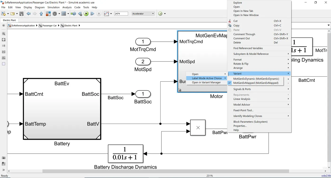
We can switch between the model types based on our application:
a) Right click on the model
b) Navigate to "Variant"
c) Navigate to "Label Active Choice"
d) Choose between the dynamic or mapped model type
STUDY 2:
To understand the theory behind calculating miles per gallon using Powertrain Blockset models and to identify the factors that are important to model fuel flow.
Powertrain blockset is a fine tool to simulate, estimate and visualize the fuel economy (mile per gallon) for different types of automotive systems. It takes a combination of the following variables as inputs (depending upon the architecture of the vehicle) for the simulation:
a) Fuel Volume Flow (as an input from engine output)
b) Vehicle Speed (as an input from the drive cycle)
c) Battery (as an input form the state of charge output)
The theory governing the calculations are as follows:
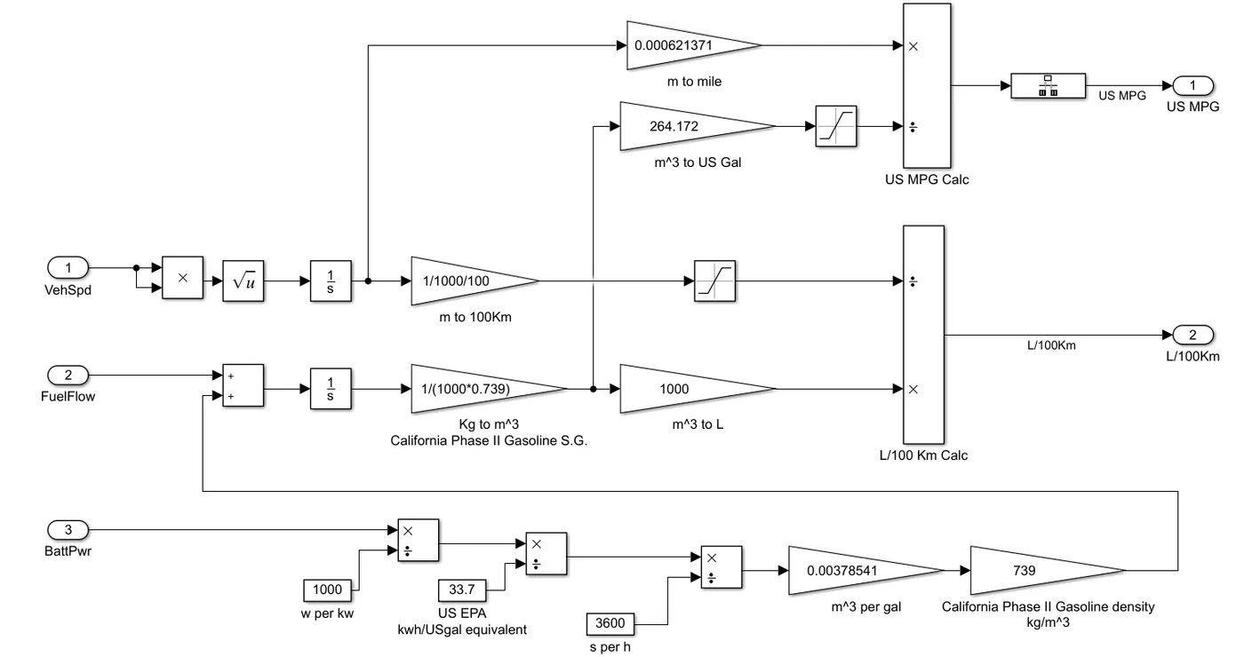
- The vehicle speed is used to calculate the total distance travelled by integrating the root mean square of the vehicle speed over the total travel time.
- If the vehicle uses fuel (eg. conventional vehicles, HEVs), the instantaneous fuel volume flow is integrated over the travel time to get accumulated fuel volume flow.
- If the vehicle used battery energy (eg. EVs, HEVs), the instantaneous battery energy is converted to the equivalent instantaneous fuel flow rate by using the standard conversion constants.
If a vehicle uses both sources of power,
`"Total instantaneous fuel volume flow" = "Fuel volume flow from engine" + "Equivalent fuel volume flow from battery"`
Thus, we can use the calculated data to calculate the MPG (conventional vehicles, HEV) or MPGe (EVs) using the simple formula:
`MPG = frac{"Distance covered" }{"Total Fuel Consumed"}`
The diagram below depicts the power calculations block for a standard hybrid vehicle which utilizes all three inputs to calculate the miles per gallon / Litres per 100 km:
STUDY 3:
To simulate the HEV Reference Application with WOT drive cycle and analysing results after changing the grade and wind velocity in the environment block.
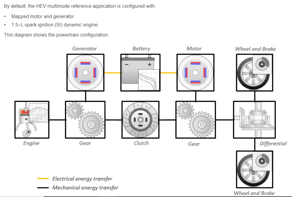
The pre-built hybrid electric vehicle model is loaded from Powertrain Blockset with the following configurations:
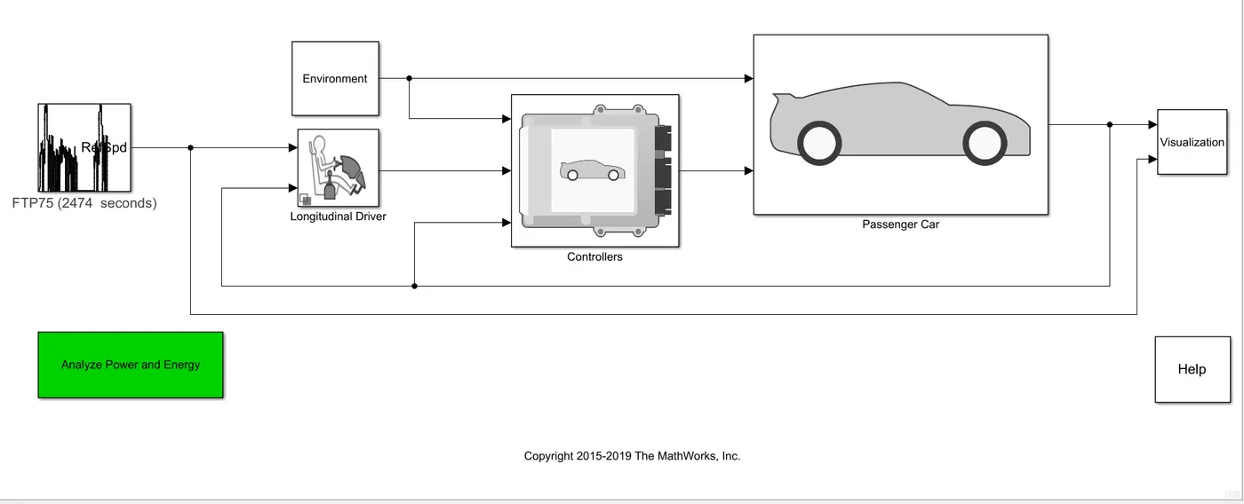
The model:
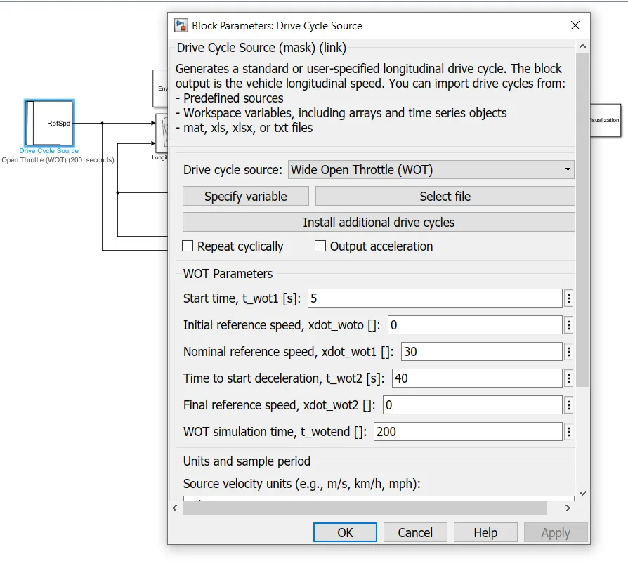
The drive cycle is changed to Wide Open Throttle mode with the following parameters:
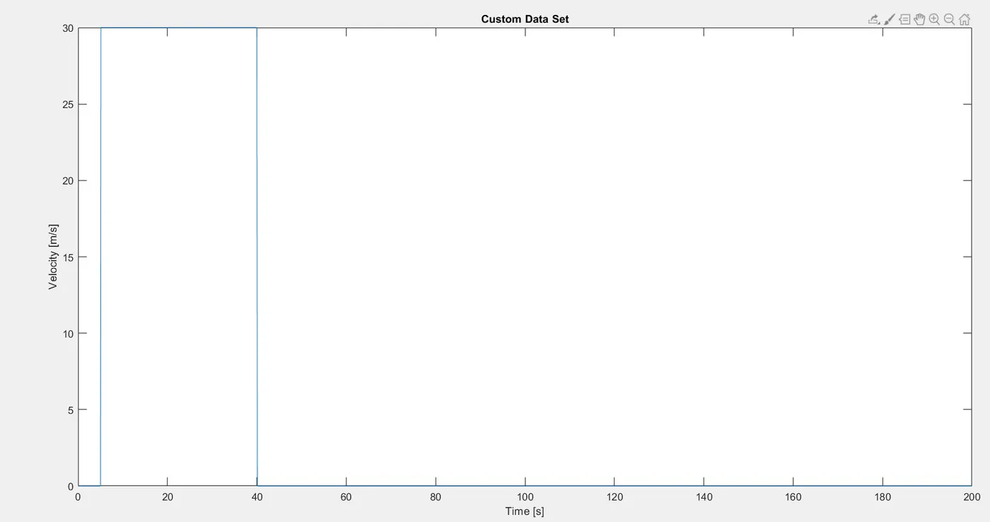
Thus, the updated drive cycle:
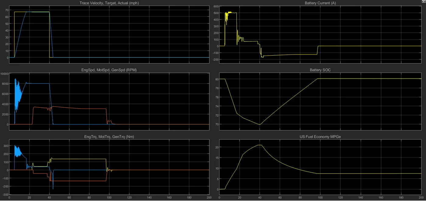
The simulation provides the following results:
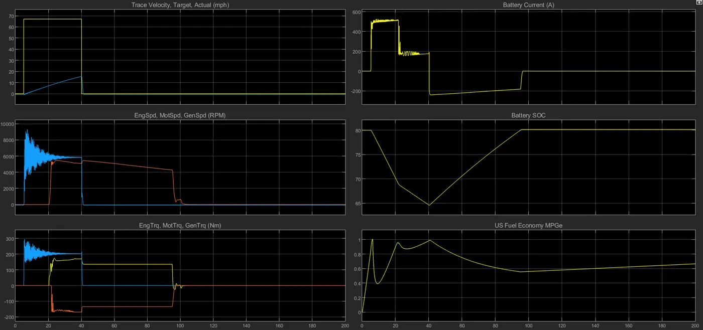
We re-run the simulation with the wind and grade parameters changed in the environement block to 20m/s and 15 degrees respectively:
Analysis:
Plot 1 (Trace Velocity vs Actual Velocity):
This plot visualizes the desired velocity from the drive cycle versus the actual velocity attained by the vehicle.
In case A, the vehicle reaches the desired velocity after a few seconds of linear acceleration.
In case B, the vehicle does not reach the desired veoocity which can be attributed to the steep gradeability and high resistance force by the wind.
Plot 2 (Engine Speed, Motor speed):
This plot visualizes the engine speed and motor speed over the drive cycle.
In case A, the the motor initiates the initial acceleration and is capable to produce enough propulsion power to reach the specified maximum velocity. However, we see the motor is activated as soon as the maximum velocity is achieved indicating that an combined effort is required to maintain the velocity. The engine continues to operate which inturn is the input for the generator for producing electricity to reach the default SOC as speicfied in the control strategy.
In case B, we observe the a similar relationship between the variables, however we observes the motor is unable to produce enough propulsion power to reach the desired velocity, thus the engine contributes to the propulsion effort. However, the combined effort is not sufficent to reach the desired velocity.
Plot 3 (Engine Torque, Motor Torque, Generator Torque):
This plot visualizes the engine torque, motor torque and generator torque over the drive cycle.
In case A, since we have a Wide-open throttle specification, the motor runs at maximum torque, however the power distribtion stabilizes between the motor and the engine as the vehicle reaches the desired velocity. A negative value for the generator indicates the engine torque is used to charge the battery as well during the propulsion time.
In case B, we observe the a similar relationship between the variables as in case A. We do not see a mutual stabilization point as the specifications of the drive cycle are not met.
Plot 4 (Battery Current):
This plot visualizes the amperage drawn from the battery over the drive cycle.
In case A, since we have a Wide-open throttle specification, the powertrain draws maximum current from the battery and stabilizes as the conditions are met and the engine is activated. A negative battery current value indicates regenerative braking and charging by the engine.
In case B, we observe the a similar relationship between the variables as in case A. However, we see that the maximum energy discharge period lasts longer indicating that the motor specifications and control strategy did not suffice to meet the specifications.
Plot 5 (SOC):
This plot visualizes the State-Of-Charge of battery over the drive cycle.
In both cases, A & B, we observe that the car starts at a SOC of 80% and continues to reduce until it reaches 65%. Thus, we can say that the control strategy specifies them as the bounds for the SOC. When the deceleration occurs, regenrative braking and the engine are used to charge the battery until 80%.
Plot 6 (Fuel Economy):
This plot visualizes the fuel economy (Miles per Gallon) over the drive cycle. It is interesting to observe that the fuel economy is less than one in case B due to the extreme enviroment conditions.
STUDY 4:
To simulate and compare the simulated results of hybrid and pure electric powertrains.
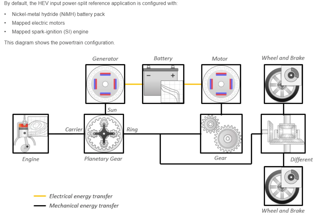
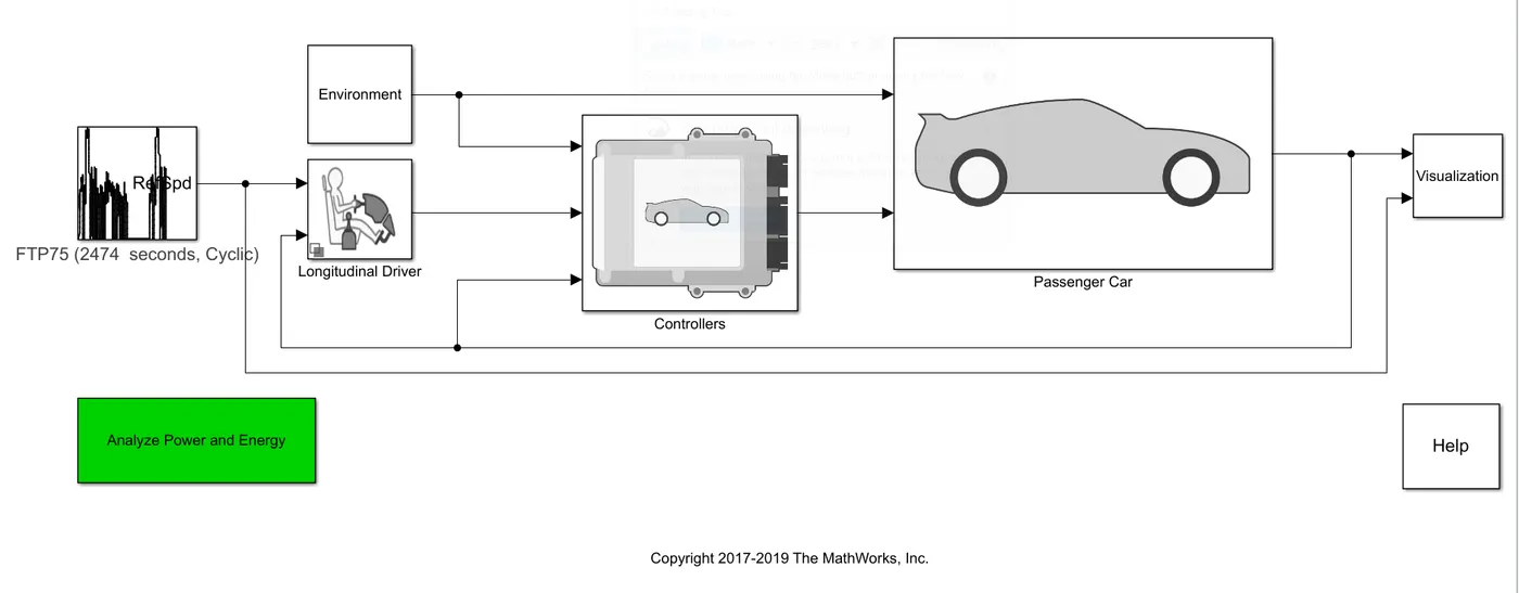
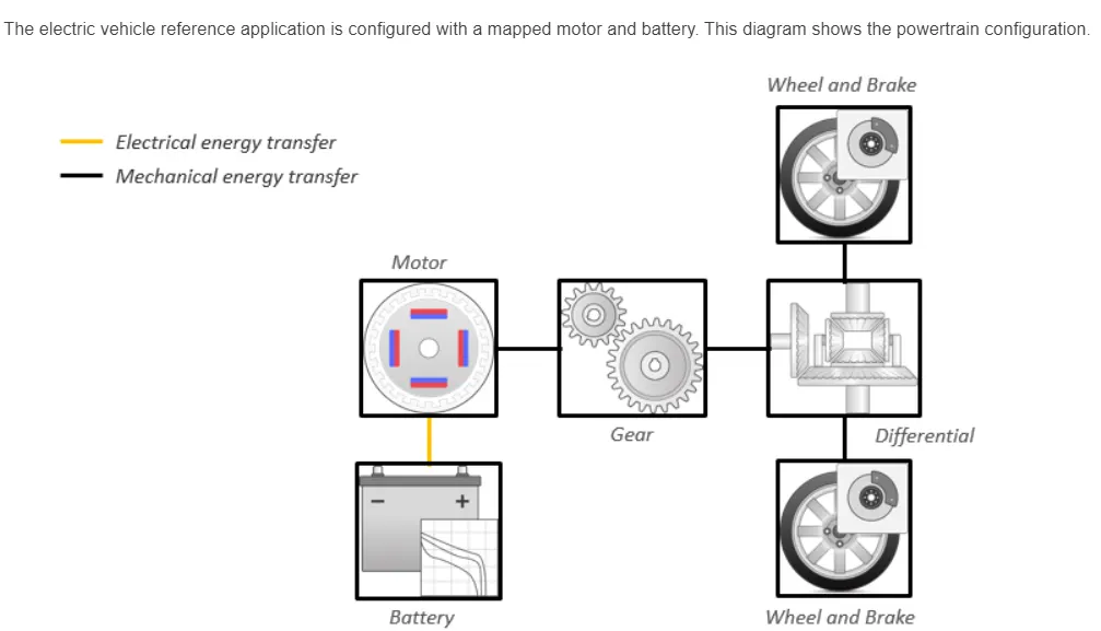
For this study we will use prebuilt models from MATLAB for our simulations. We will compare an input power-split HEV (commonly found in Toyota PRIUS) against a pure electric powertrain along a FTP75 drive cycle.
a) Input power-split HEV:
Configuration:
SIMULINK model:
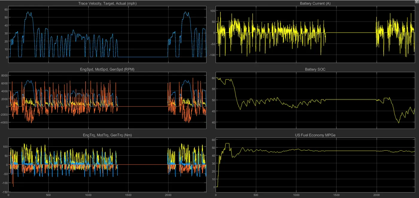
Simulation results:
b) Pure electric vehicle:
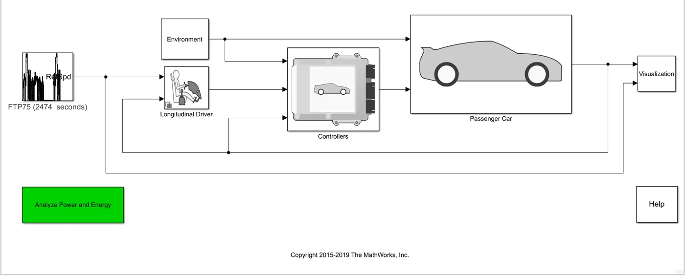
Configuration:
SIMULINK model:
Simulation results:
Analysis:
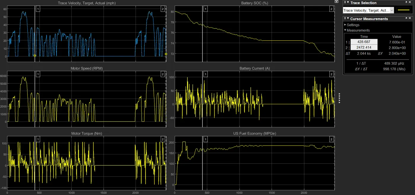
Since we are comparing an electric vehicle against an hybrid electric vehicle, it is important to have a level playing field. Thus, we run the vehicle along the same drive cycle and compare variables that are important to the consumer and the environment i.e. efficiency, range and MPGe.
From the outset, the EV seems a clear winner due to the larger MPGe in this study. This is attributed to the fact that the HEV uses a nickel metal hydride chemistry whereas the EV uses a Li-Ion chemistry which has a superior energy density and lower discharge rate. That being said, when compared over multiple cycles HEV has the edge over an EV due to its ability to use fuel for propulsion which has a high specific energy density thus provivng longer ranges in practical applications.