Introduction to HEV using MATLAB and SIMULINK: Wide-Open Throttle (#02)

AIM:

The aim of this challenge is to compare the hill climbing power required by a loaded and partially-loaded by a Tata Ultra Truck and to find dimensions of a flyover meeting certain specification. We also aim to prepare a drive cycle and using it in a SIMULINK model to calculate hill-climbing force and modeling a Wide-Open Throttle (WOT) response for a GM EV1.

OBJECTIVES:

1. To find the ratio of hill-climbing power for a loaded and partially-loaded TATA Ultra T-16s truck.

2. To find the minimum length of a flyover that has a minimum summit height of 5.5 meters.

3. To create a new drive drive cycle with gradeability. Use this in SIMULINK to calculate hill-climbing force.

4. To model a WOT (Wide Open Throttle) response of GM EV1 car and comparing it with the official figures of the performance of a real vehicle.

STUDY 1:

To find the ratio of hill-climbing power for a loaded and partially-loaded TATA Ultra T-16s truck.

The specifications of the vehicle are provided on their official website: https://light-trucks.tatamotors.com/light-trucks/tata-ultra/specifications/tata-ultra-t-16s-light-trucks-specifications.aspx

Since considering the extreme situations is vital to vehicle design, I have assued the hill-climbing gradeability as 26.7%.

The hill-climbing force is calculated as Fhc=m⋅g⋅sin(ψ)">Fhc=m⋅g⋅sin(ψ)Fhc=m⋅g⋅sin(ψ)

The resultant hill climbing power is calculated as Phc=Fhc⋅v">Phc=Fhc⋅vPhc=Fhc⋅v, where v">vv is the velocity of the truck

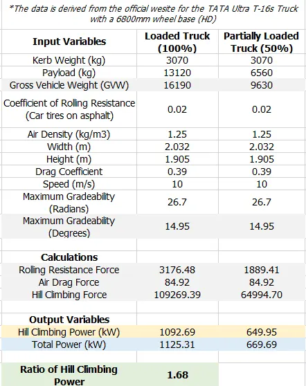
The excel sheet can be found in the zip folder as "Study 1"

STUDY 2

Gradeability is a vital considerations when designing vehicles capable of transporting payloads. Since our goal is to find the minimum length of the flyover we need to use the maximum gradeability which is 26.7% = 14.95o">14.95o14.95oas stated by the manufacturer. We use this as a reference to do our calculations.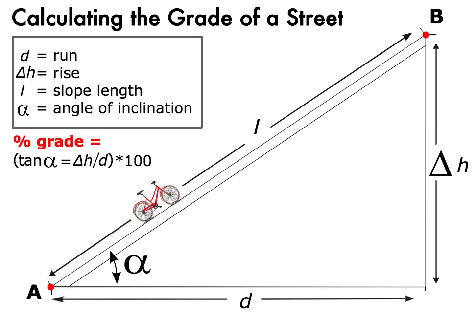

Since we need the minimum summit to be 5.5 meters, we use sin(ψ)=heighthypotenuse">sin(ψ)=heighthypotenusesin(ψ)=heighthypotenuse

Thus, hypotenuse=heightsin(ψ)">hypotenuse=heightsin(ψ)hypotenuse=heightsin(ψ) ⇒">⇒⇒hypotenuse=5.5sin(14.95)">hypotenuse=5.5sin(14.95)hypotenuse=5.5sin(14.95) ⇒">⇒⇒ hypotenuse=21.32">hypotenuse=21.32hypotenuse=21.32

Thus the length of the flyover should be 21.32m">21.32m21.32m.

Now, we can use adjacent=heighttan(ψ)">adjacent=heighttan(ψ)adjacent=heighttan(ψ) ⇒">⇒⇒ adjacent=20.60">adjacent=20.60adjacent=20.60

Thus, the run of the flyover should be 20.60m">20.60m20.60m

STUDY 3:

In this study, the goal is to create a new drive cycle in MS Excel as velocity-time data points with gradeability. We use this data to find the hill climbing force experienced by the vehicle and the impact of this force on the velocity of the vehicle.

We use the pre-existing Driver_Glider model from MATLAB and Simulink Racing Lounge: Vehicle Modeling package.

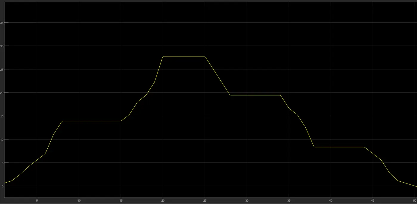
The drive cycle is as follows:

Time	Velocity (m/s)	Velocity (kmph)	Angle (Degrees)	Radian
0	0.00	0	0	0.00
1	0.56	2	0	0.00
2	1.11	4	0	0.00
3	2.50	9	0	0.00
4	4.17	15	0	0.00
5	5.56	20	0	0.00
6	6.94	25	0	0.00
7	11.11	40	0	0.00
8	13.89	50	0	0.00
9	13.89	50	0	0.00
10	13.89	50	0	0.00
11	13.89	50	0	0.00
12	13.89	50	0	0.00
13	13.89	50	0	0.00
14	13.89	50	0	0.00
15	13.89	50	0	0.00
16	15.28	55	26.7	0.47
17	18.06	65	26.7	0.47
18	19.44	70	26.7	0.47
19	22.22	80	26.7	0.47
20	27.78	100	26.7	0.47
21	27.78	100	0	0.00
22	27.78	100	0	0.00
23	27.78	100	0	0.00
24	27.78	100	0	0.00
25	27.78	100	0	0.00
26	25.00	90	0	0.00
27	22.22	80	0	0.00
28	19.44	70	10	0.17
29	19.44	70	10	0.17
30	19.44	70	10	0.17
31	19.44	70	10	0.17
32	19.44	70	10	0.17
33	19.44	70	10	0.17
34	19.44	70	10	0.17
35	16.67	60	0	0.00
36	15.28	55	0	0.00
37	12.50	45	0	0.00
38	8.33	30	0	0.00
39	8.33	30	0	0.00
40	8.33	30	0	0.00
41	8.33	30	0	0.00
42	8.33	30	0	0.00
43	8.33	30	0	0.00
44	8.33	30	0	0.00
45	6.94	25	0	0.00
46	5.56	20	0	0.00
47	2.78	10	0	0.00
48	1.11	4	0	0.00
49	0.56	2	0	0.00
50	0.00	0	0	0.00

The excel sheet can be found in the attached zip folder as "Study3"

The final Driver_Glider model is as follows:

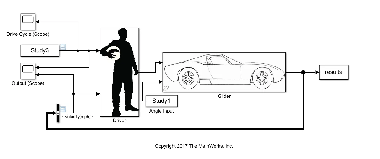
The following changes were made to the glider model to find the hill climbing force as a function of inputted inclination angle:

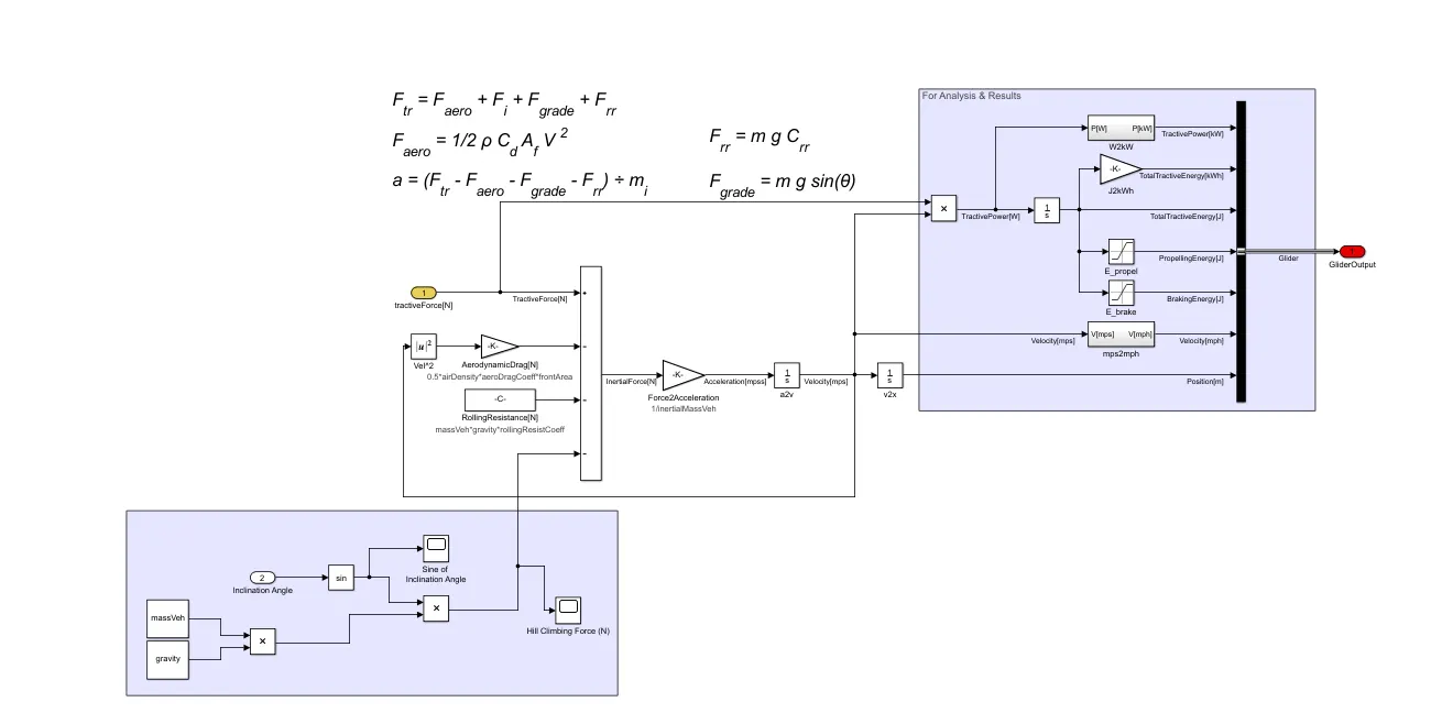
INPUTS: 1) Drive Cycle - Imported from MS Excel as a numeric matrix

2) Inclination Angle (in radians) - Imported as a numeric matrix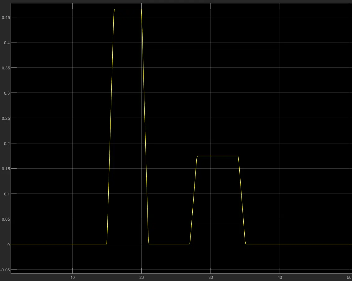

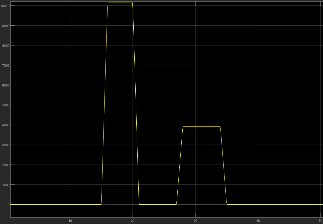
OUTPUT:

1) Hill Climbing Force

2) Impact on Velocity of vehicle due to gradeability: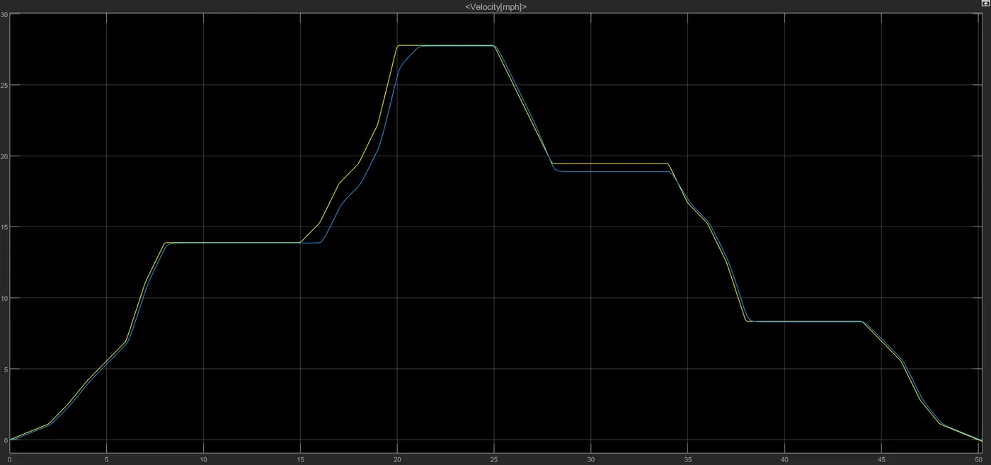

STUDY 4:

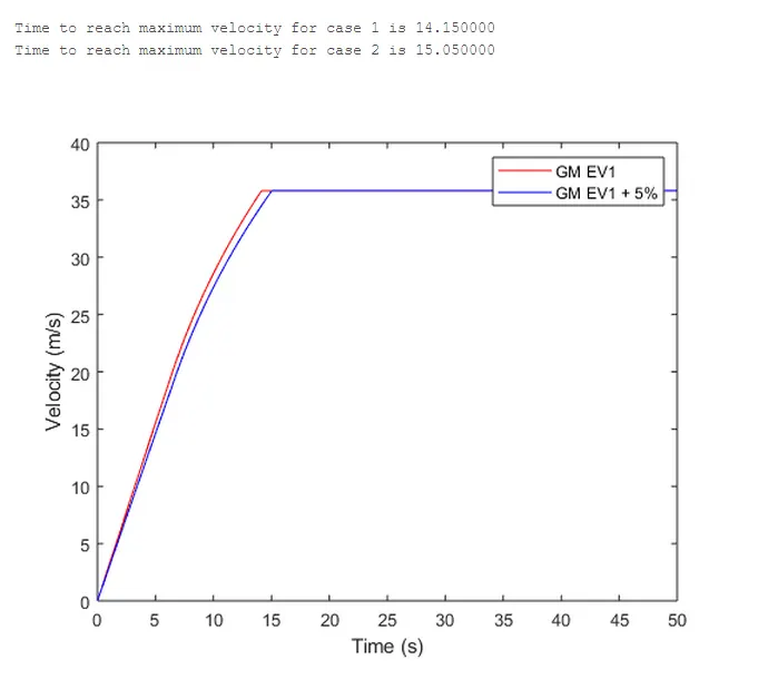
In this study we aim to model a WOT (Wide Open Throttle) response of GM EV1 car and comparing it with the official figures of the performance of a real vehicle. We then change each of the parameters by 5% and compare it with the original response.

*The data is derived from various sources on the internet
Input Variables	GM EV1	GM EV1 (+5%)
Kerb Weight (kg)	1400	1470
Payload (kg)	140	147
Gross Vehicle Weight (GVW)	1540	1617
Adjusted GVW	1560	1638
Coefficient of Rolling Resistance (Car tires on asphalt)	0.0048	0.00504
Air Density (kg/m3)	1.25	1.25
Frontal Area (m2)	1.8	1.89
Drag Coefficient	0.19	0.19
Gear Ratio (G)	11	11.55
Maximum Torque (Nm)	140.00	140
Radius of tire (m)	0.30	0.315
Motor-Axle Coupling efficiency	0.95	0.95
Critical velocity of vehicle (m/s)	19.80	19.8
Maximum Velocity of Vehicle	35.76	35.76

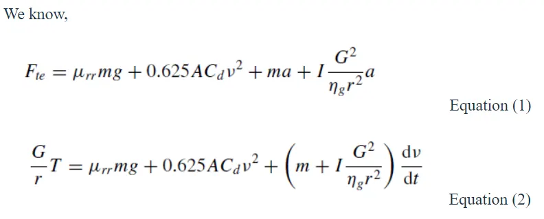
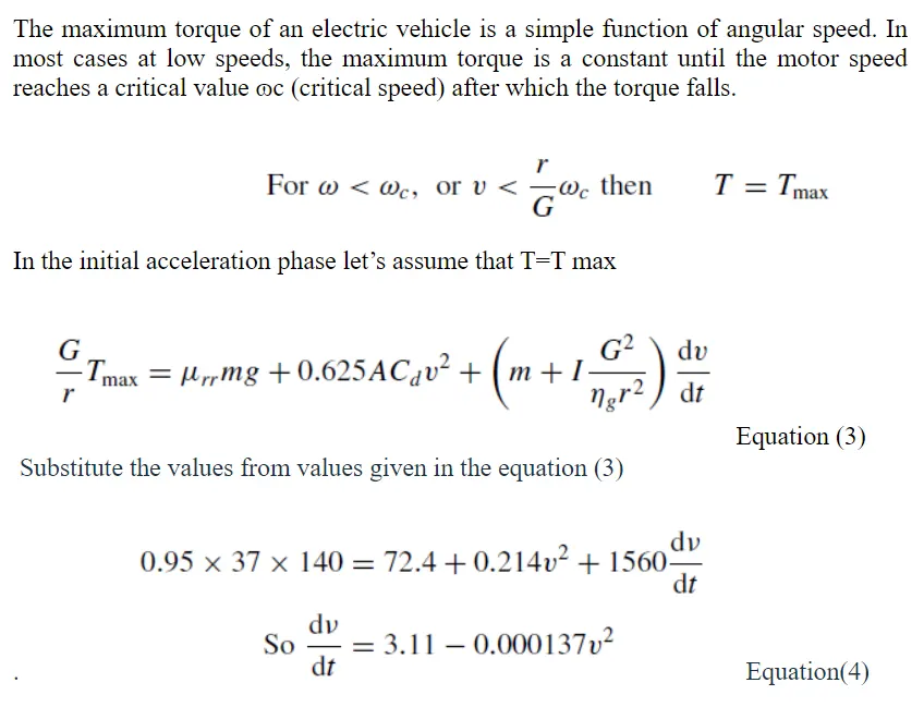
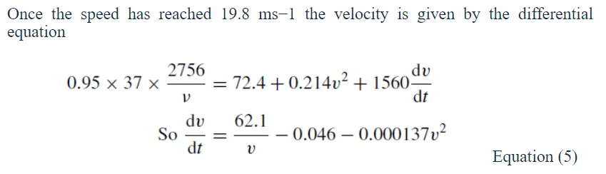
For case 1,

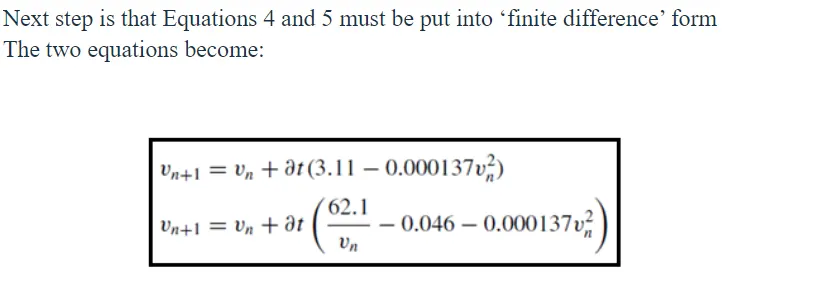
Similarly for case 2, the equations become: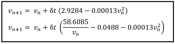

We will use MATLAB to solve the above equations to find the change in acceleration time the electric vehicle for :

clc
clear all
close all

t = linspace (0,50,1001); % a time vector from 0 to 50 with equally spaced 1000 data points

v_1 = zeros(1,1001); % zero vector for velocity calculated in case 1
v_2 = zeros(1,1001); % zero vector for velocity calculated in case 2

dT = 50/1000; % smallest time interval

%CASE1

for n = 1:1000
    if v_1(n) < 19.8
        v_1(n+1) = v_1(n) + dT * (3.11 - 0.000137 * (v_1(n)^2));
    elseif v_1(n) >= 35.76
        v_1(n+1) = v_1(n);
    else
        v_1(n+1) = v_1(n) + dT * ((62.1/v_1(n)) - 0.046 - 0.000137 * (v_1(n)^2));
    end
end

%CASE2

for n = 1:1000
    if v_2(n) < 19.8
        v_2(n+1) = v_2(n) + dT * (2.9284 - 0.00013 * (v_2(n)^2));
    elseif v_2(n) >= 35.76
        v_2(n+1) = v_2(n);
    else
        v_2(n+1) = v_2(n) + dT * ((58.6085/v_2(n)) - 0.0488 - 0.00013 * (v_2(n)^2));
    end
end

% Plotting the velocity-time graphs

plot (t,v_1,'color','r')
hold on
plot (t,v_2,'color','b')
xlabel ('Time (s)')
ylabel ('Velocity (m/s)')
legend ('GM EV1','GM EV1 + 5%')
hold off

%Finding acceleration time 

for n=1:1000
    if (v_1(n) == v_1(n+1))
        fprintf('Time to reach maximum velocity for case 1 is %f',t(n))
        break
    end
end

for n=1:1000
    if (v_2(n) == v_2(n+1))
        fprintf('nTime to reach maximum velocity for case 2 is %f',t(n))
        break
    end
end

OUTPUT: