Week 4.2: Project - Transient simulation of flow over a throttle body

Aim:-Transient simulation of flow over a throttle body

objective:-

Setup and run transient state simulation for flow over a throttle body.

Post process the results and show pressure and velocity contours.

Show the mesh (i.e surface with edges)

Show the plots for pressure, velocity, mass flow rate and total cell count.

Also show the calculations on how you calculated an end time for the simulation.

Create an animation in which it throttle movement should be visible.

throttle body:

A throttle is the mechanism by which fluid flow is managed by constriction or obstruction.

An engine's power can be increased or decreased by the restriction of inlet gases (by the use of a throttle), but usually decreased. The term throttle has come to refer, informally, to any mechanism by which the power or speed of an engine is regulated, such as a car's accelerator pedal. What is often termed a throttle (in an aviation context) is also called a thrust lever, particularly for jet engine powered aircraft. For a steam locomotive, the valve which controls the steam is known as the regulator.

the throttle body is the part of the air intake system that controls the amount of air flowing into the engine, in response to driver accelerator pedal input in the main. The throttle body is usually located between the air filter box and the intake manifold, and it is usually attached to, or near, the mass airflow sensor. Often, an engine coolant line also runs through it in order for the engine to draw intake air at a certain temperature (the engine's current coolant temperature, which the ECU senses through the relevant sensor) and therefore with a known density.

transient simulation of throlttle body

Transient models, however, can handle conditions that change with time and assess the time-dependent impact on thermal and flow predictions.

need for transient simulation: It is obvious that transient simulations are vital when evaluating scenarios that are fundamentally dynamic.

transient multiphase flow simulations may become relevant as the conditions change over time.

transient simulation of pipe flow may be crucial even for scenarios where the configuration of the system is considered constant. In cases with a fixed separator pressure, constant valve openings, set pump speeds, steady ambient conditions, etc. it may be tempting to apply a steady state simulation approach. However, just because the system itself is unchanging, the multiphase flow may still be unstable. A steady state simulator will generally be able to predict various flow regimes, for example the time-averaged behavior of hydrodynamic slug flow, and may even have correlations for estimation of slug statistics built in. However, such predictions are, by design, inferior to transient physics-based simulations, which can predict liquid loading and local liquid accumulation over time, terrain-induced flow instabilities, as well as other flow dynamics and thermal transients.

simulation setup:-

open converge application import stl file check the diagnossis if any error present try to resolve them then define boundaries and name them accordingly and select normal toggle make sure the normal is interior to the elbow

now diaganos the workpiece again

case setup

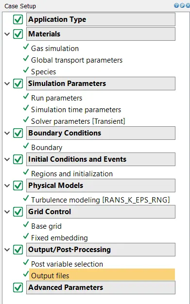
appication type:- time based

materials : air as predefined mixture

Simulation parameter:

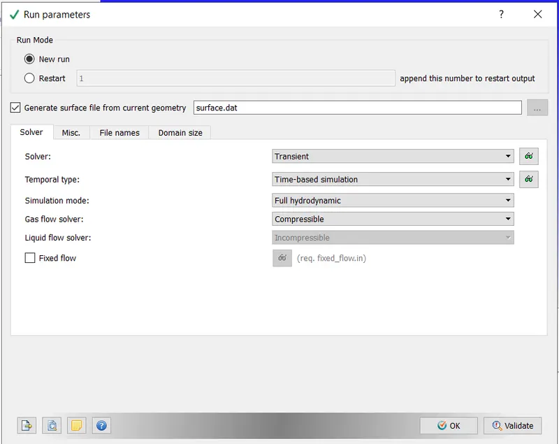
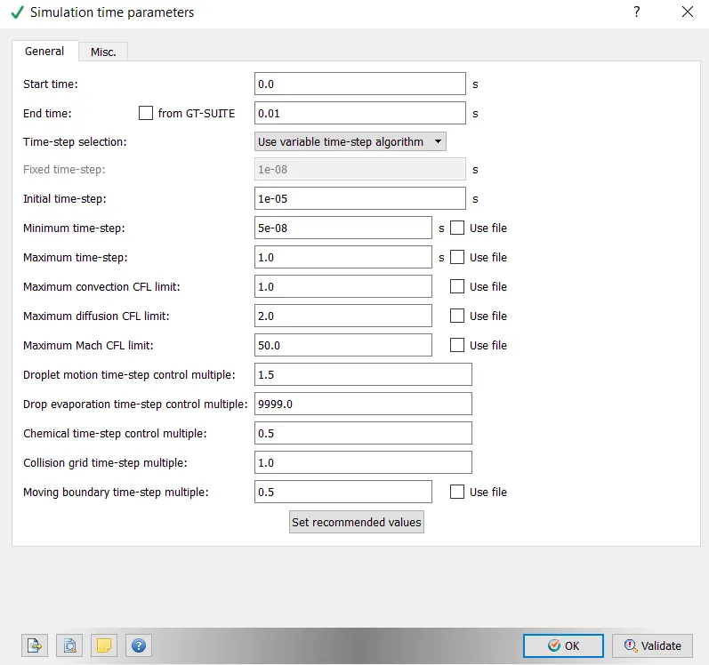
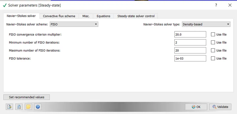
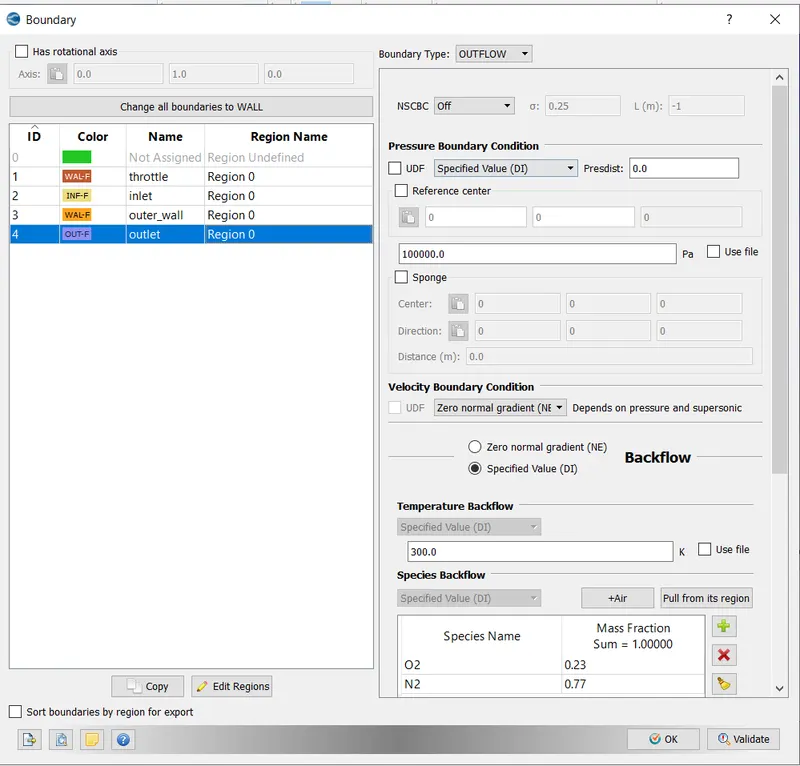
boundary condition:

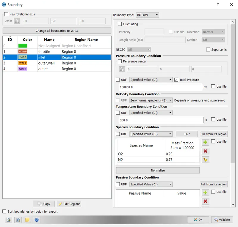
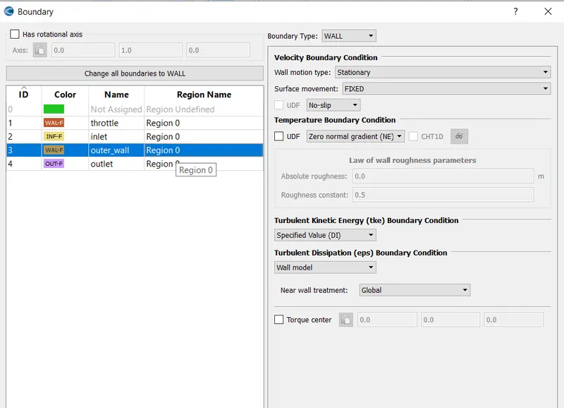
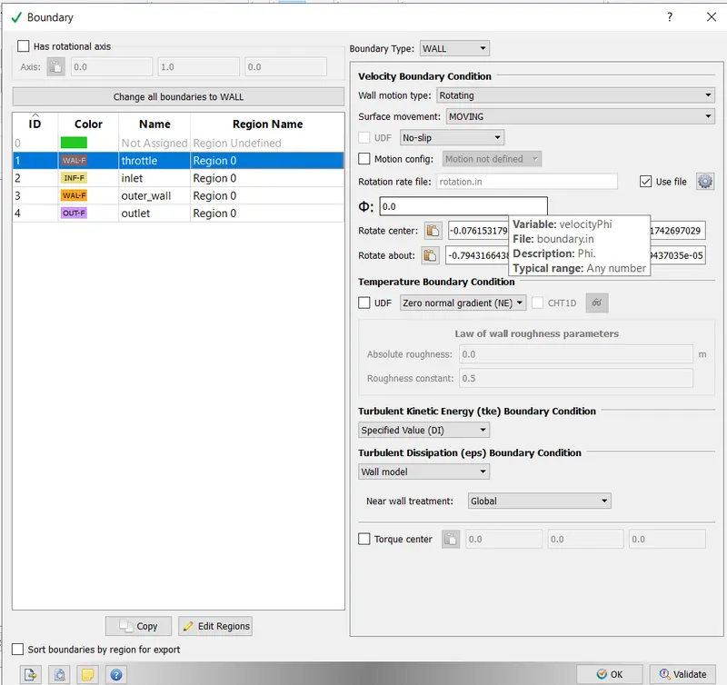
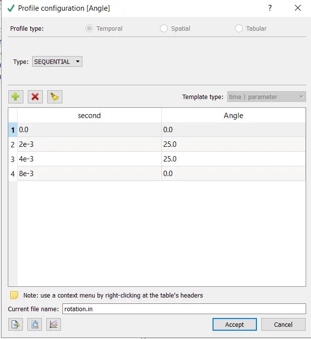
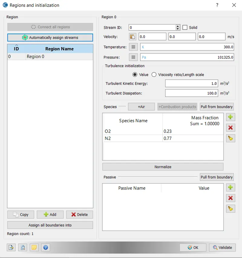
region and intialization:

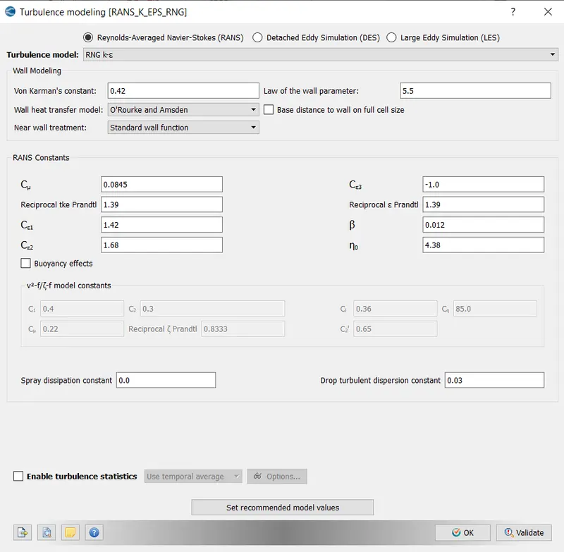
turbulne model:-

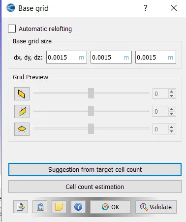
grid control:-

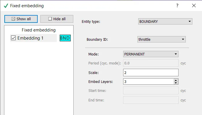
output/post processing:-

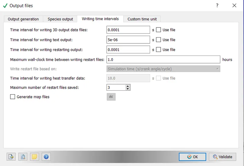
after case set up valicate the setup if there is no error then export the input file to a folder

now open cygwin and navigate to that perticular folder and run the this commnad

mpiexec.exe -n 6 converge.exe restricted

wait till simulaton complete

the go to converge studio post processing to convertthe post processing files to reable file for paraview to look into postprocessing

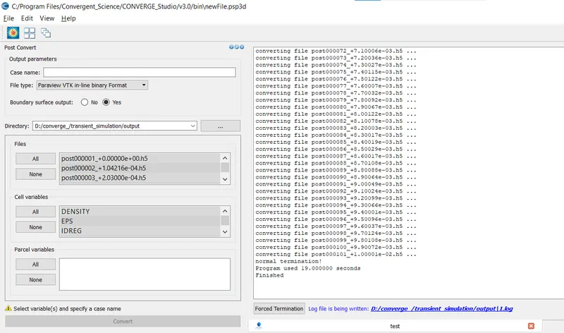
now open paraview apllication to see the post processing

result:-

plots

after simulation look for plots in converge studio application in line plotting section

some of the plots shown here

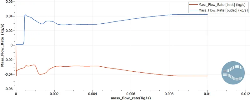
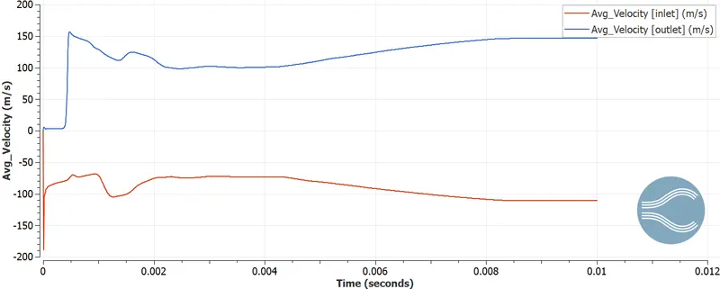
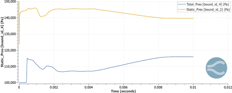
mass flow rate, velocity and pressure at inlet and outlet

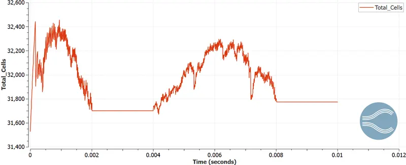
cell count

post processing

to see post processing result open paraview application

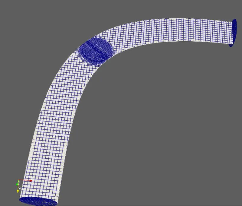
mesh

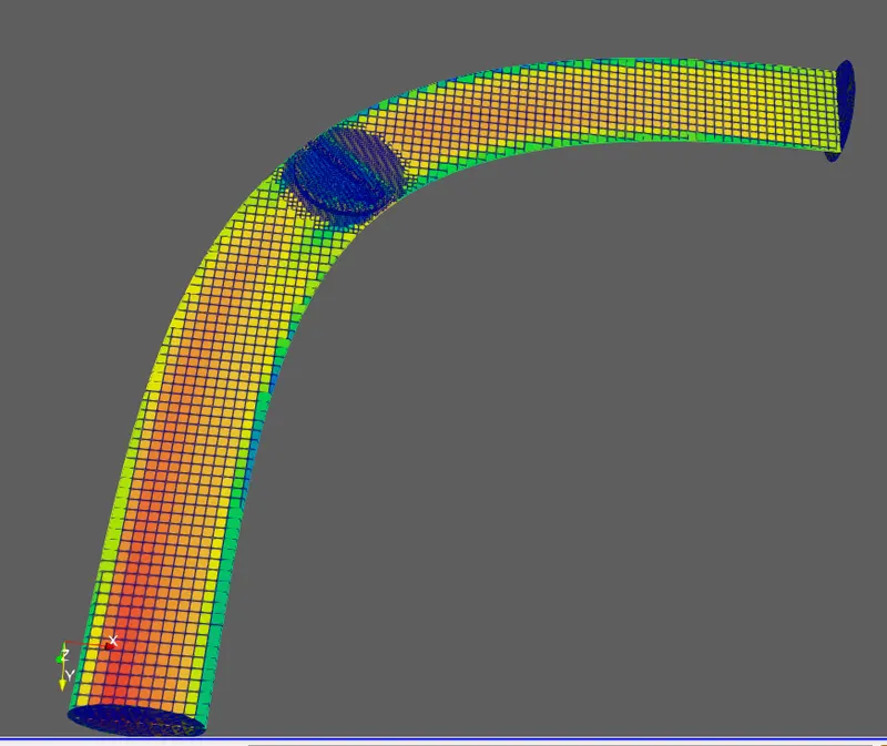
velocity

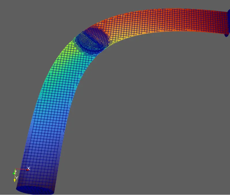
pressure

conclusion:

from mass flow rate, velocity plot result it can be seen that at outlet intially till time 2 ms there is drop this id due because at this time the throttle is clossing due to this there is a drop in velocity and mass flow rate

after 2ms t 4 ms the mass flow rate and velocity is constant because the throttle wall is closed

after 8m ms the throttle wall is gradually opening so doe increase in velociy and mass flow rate

even there is increase and decrease in cell count this because while throttlr movemet there is change mesh

the animation which support the conclusion is attached in zip file inclusding converge set up and paraview setup