Week 4.1 - Solving second order ODEs

Solving second order ODEs.

Aim: To slove second order ordinary order Ordinary Differential Equation that describes the position of the "ball" w.r.t time.

(simple pendulam).

Objective: ODE represents the equation of motion of a simple pendulum with damping.

Theory:

The period of a pendulum does not depend on the mass of the ball, but only on the length of the string. Two pendula with different masses but the same length will have the same period. Two pendula with different lengths will different periods; the pendulum with the longer string will have the longer period.

How many complete oscillations do the blue and brown pendula complete in the time for one complete oscillation of the longer (black) pendulum?

From this information and the definition of the period for a simple pendulum, what is the ratio of lengths for the three pendula?

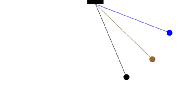
With the assumption of small angles, the frequency and period of the pendulum are independent of the initial angular displacement amplitude. A pendulum will have the same period regardless of its initial angle. This simple approximation is illustrated in the animation at left. All three pendulums cycle through one complete oscillation in the same amount of time, regardless of the initial angle.

Equation used

`dθ2dt=[−bm.(θ2)−glsinθ1]dθ2dt=[-bm.(θ2)-glsinθ1]`

Given data:

simulation the motion 15 sec

m = 1kg

b = 0.05 damping cofficient

g = 9.81 m/s

l in meter

clear all
close all
clc

b = 0.05;
g = 9.81;
l = 1;
m = 0.1;
% initial condition
theta_0 = [0;5];
% time points
t_span = linspace(0,10,500);
%solve ode
[t,result] = ode45(@(t,theta)ode_func(t,theta,b,g,l,m),t_span,theta_0);
plot(t,result(:,1))
hold on
plot(t,result(:,2))
xlabel('time')
ylabel('velocity')
title('ode45_687');
grid on
hold off
displacement = result(:,1);
velocity = result(:,2);
%fixed coordinate
x0 = 1;
y0 = 1;
ct = 1;
for i = 1:length(displacement)
% coordinate
x1 = 1-l*sin(displacement(i));
y1 = 1-l*cos(displacement(i));

figure(2)
%plot fixed link
plot([0 2 ],[1 1],'linewidth',15,'color','b')
hold on
plot([1 x1],[1 y1],[x1 x1],[y1 y1],'-o','markersize',25,'markerfacecolor','g','linewidth',4)
plot(x0,y0,'-o','markersize',3,'markerfacecolor','b')
%axis setting
axis([0 2 -0.5 2])

M(ct) = getframe(gcf);
ct = ct+1;
hold off
end
movie(M)
Videofile = VideoWriter('ode_45.avi','uncompressed AVI');
open(Videofile)
writeVideo(Videofile,M)
close(Videofile)

function code

function[dtheta_dt] = ode_func(t,theta,b,g,l,m)
theta1 = theta(1)
theta2 = theta(2)
dtheta1_dt = theta(2);
dtheta2_dt = -(b/m)*theta2-(g/l)*sin(theta1);
dtheta_dt = [dtheta1_dt; dtheta2_dt];
end

plot the result velocity v/s time.

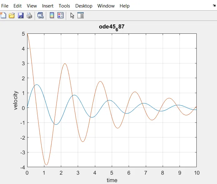
simple pendulum

https://drive.google.com/file/d/1zjt1zIO8MLgUPRbk3z1wXP_NgvddJOo-/view?usp=sharing