Week 4.1 - Solving second order ODEs

Aim :- Write a program in Matlab that will simulate the pendulum motion.

Objective :-

1. Is to write a program that solves the following ODE.
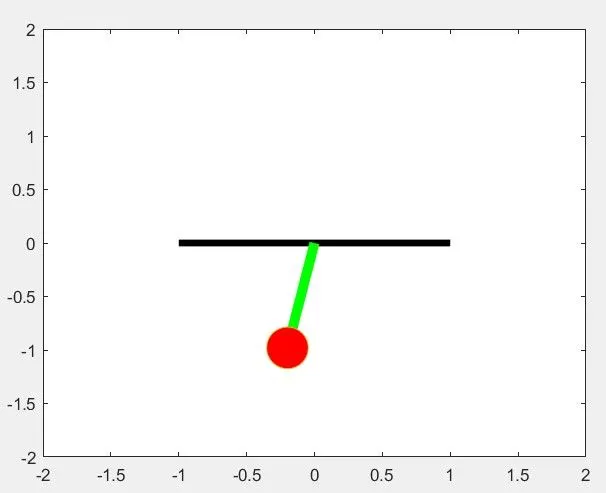
2. To create an annimation movies to show pendulum movment.

Introduction :-

What is ODE (Ordinary Differential Equation) ?

• In mathematics, an ordinary differential equation (ODE) is a differential equation containing one or more functions of one independent variable and its derivatives.
• The two important aspects of ordinary differential equations, is the Order and Degree of an differential equation.
• In this Challenge we are going to use Second order ODE. This ODE represents the equation of motion of a simple pendulum with damping `(d^2theta)/dt^2 + (b)/(m)*(d theta)/(dt) + (g)/(L) sin theta = 0`

In the above equation,

g = gravity in m/s2,

L = length of the pendulum in m,

m = mass of the ball in kg,

b= damping coefficient.

Given values for above listed parameters are as follow -

L=1 metre,

m=1 kg,

b=0.05.

g=9.81 m/s2.

Simulate the motion between 0-20 sec,

for angular displacement=0, angular velocity=3 rad/sec at time t=0.

Function code :

function [dtheta_dt] = ode_func(t,theta,b,g,l,m)
theta1 = theta(1);
theta2 = theta(2);
dtheta1_dt = theta2;
dtheta2_dt = -(b/m)*theta2-(g/l)*sin(theta1);
dtheta_dt = [dtheta1_dt ; dtheta2_dt]
end

Code Explanation -

1. Ode_func is the function definition with the input arguments for the statement which we are used in the main code with ode45 as inbuild solver.
2. The input arguments for ode function are time, theta which is our solution array, damping coefficient (b), gravity(g), length(L) and mass(m).
3. Theta1 and theta2 is our solving array values for Theta which is used in ode function.
4. Then defining first ode equation that is dtheta1_dt = thata2
5. After that define second ode (dtheta2_dt) with parameters used solve second order ode for a pendulum movement.
6. Then we combine the both ode in an array form by using semi-colon between them.

Code For Solving ODE:

clear all
close all
clc

%Input values 
%damping coefficient 
b = 0.05;

%gravity m/s^2
g = 9.81;

%length in mtr
l = 1;

%mass in kg
 m = 1;
 
 %initial condition 
 theta = [0;3];
 
 %time points 
 t_span = linspace(0,20,300);
 
 %solvind ODE%
 [t,results] = ode45(@(t,theta) ode_func(t,theta,b,g,l,m),t_span,theta);
 
%Plotiing second order ODE 
figure(1)
 plot(t,results(:,1))
 hold on
 plot(t,results(:,2))
 grid on
 xlabel('Time')
 ylabel('Dispalcement & Velocity')
 
 %Animation 
  ct = 1;
  theta_1 = results(:,1);
 for i = 1:length(results(:,1))
     x0 =0;
     y0 = 0;
     theta_2 = theta_1(i)
     
     x1 = l*sin(theta_2);
     y1 = -l*cos(theta_2);
     
     %Plotting Annimation 
     figure(2)
     plot([-1,1],[0,0],'linewidth',4,'color','k')
     hold on
     plot([x0 x1],[y0 y1],'linewidth',6,'color','g')
     hold on
     plot(x1,y1,'o','markersize',25,'markerfacecolor','r')
     axis([-2 2 -2 2])
     hold off
     pause(0.01)
     
     M(ct) = getframe(gcf);
     ct= ct+1;
 end
 
 %Converting the annimation into movie
 movie(M)
 videofile = VideoWriter('Pendulum.avi','Uncompressed AVI');
 open(videofile);
 writeVideo(videofile,M);
 close(videofile);

Code Explanation-

1. Using the given values of b, m, l and g assign input parameters to solve second order ODE.
2. Assign value to the theta for initial condition that is nothing but Angular Displacement = 0 and Angular Velocity = 3 rad/sec.
3. For simulating the pendulum motion used time span between 0 – 20 sec.
4. Our next step in code is solving ODE, so to store the result of solved ode we assign name to the function as t and results because we are using two thetas which is in array.
5. T for storing the integration time and results which is column vector storing two parameters are velocity and displacement.
6. Use ode45 which is the inbuild solver and (t, theta) are the main inputs to the ode function with calling our main function.
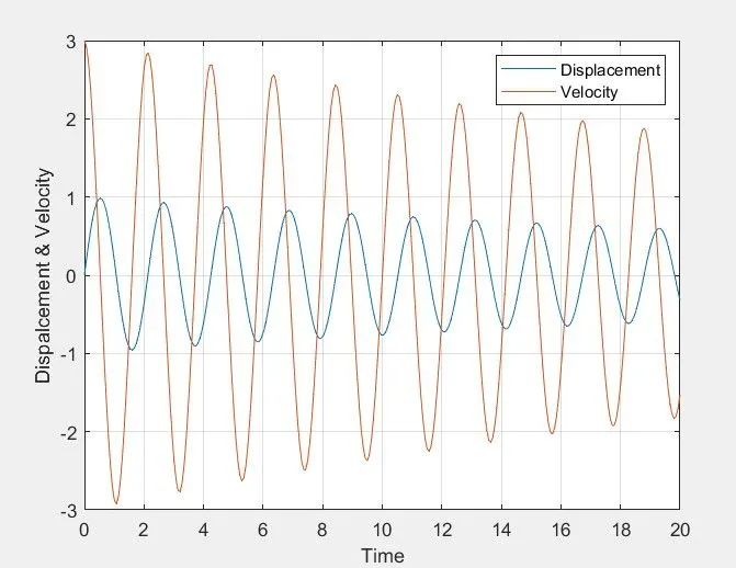
7. Finally using plot command we can observe the curve which is of displacement and velocity with respect to time.
8. So, after getting the required result we are moving forward to create an animation movie for pendulum movement and save it.
9. To capture the frames to create movie (ct) is used to capture the current frames.
10. Using for loop calculated all the axis values and plotting the pendulum lines.

Error faced –

Error - I had faced an error which is showing permission denied for saving animation movie i.e. Pendulum AVI.

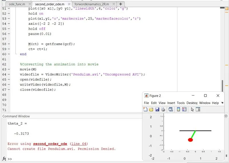
Solution – To resolve this error I had changed the directory path of the code files to another location then after running the code matlab saved the animation movie in the new directory path location.

Results :-

1) After the code for solving Second order ODE we get the output which display the relation between Time with respect to Angular Velocity and Displacement.

2) Pendulum movemet to display relation between moving ball w.r.t. time.The annimation movie is uploaded at you -tube and here is the link to see the result.

https://youtu.be/c2a0kktNwhk