SOLVING SECOND ORDER ODE

A differential equation that consists of a function and its second-order derivative is called a second order differential equation.

Mathematically, it is written as

(d²θ/dt²) ⁺ (b/m) (dθ/dt) + (g/l) (sinθ) = 0

Let’s simplifying the above equation

Put θ = θ₁

Therefore, dθ/dt = dθ1/dt and dθ1/dt = θ2 ------------(1)

(d²θ/dt²) = (d²θ₁/dt²) = (d/dt) (dθ₁/dt) = (d/dt) (θ2) --------------(2)

Now putting the values from equation (1) and (2) in above equation,

We get,

(d²θ₁/dt²) + (b/m) (dθ₁/dt) + (g/l) (sinθ₁) = 0

(dθ₂/dt) + (b/m) (θ₂) + (g/l) (sinθ₁) = 0

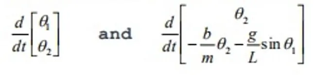
(dθ₂/dt) = - (b/m) (θ₂) - (g/l) (sinθ₁)

Therefore, the second order ODE in matrix form is

Second-Order Differential Equations as Systems

Every second-order differential equation may be considered as a system of two first-order equations. This has a number of uses. In particular, it enables us to use first-order numerical methods to approximate the solution of a second-order initial value problem.

In order to have a particular example, let's consider the second-order equation describing the motion of a pendulum.

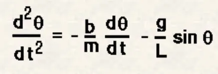
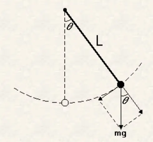
Here θ is the angle the pendulum has moved from the vertical, L is the length of the pendulum, g is the acceleration due to gravity, m is the mass of the pendulum, and b is a damping coefficient. See the figure below.

_{Matlab Program for Second order ODE and creating Pendulum Animation}

clear all
close all
clc
 
% considering the values for input variables
b= 0.05 % damping co-efficient
g = 9.81 % gravity m/s^2 
l = 1 % length of spring in m
m = 1 %mass of the bob in kg

%definig initial conditions for displacement and velocity
theta_0 = [0;6]
% time span of pendulum as it oscilates 
t_span = linspace(0,20,500)
%solving ODE
[t,results] = ode45(@(t,theta) ode_func(t, theta, b,g,l,m), t_span, theta_0);

%plotting the graph
figure(1)
hold on
plot(t,results(:,1))
plot(t, results(:,2))
title('damped harmonic motion for pendulum')
legend('angular displacement','angular velocity')
ylabel('plot')
xlabel('time(s)')

ct = 1; 
for i =1:length(results(:,1))
    x_start = 0
    y_start = 0
    x_end = l*sin(results(i,1))
    y_end = -1*cos(results(i,1))
    
    figure(2)
    plot([-1 1],[0,0],'linewidth',5)
    hold on
    plot([x_start x_end],[y_start y_end],'linewidth',3)
    hold on
    
    plot(x_end, y_end,'o' , 'markersize',15,'markerFacecolor','y')
    title('Animation for Oscillating pendulum')
    axis([-1.5 1.5 -1.5 1])
    pause(0.02)
    hold off
    
    M(ct)=getframe(gcf)
    ct = ct+1
end
% creating movie for pendulum
movie(M)
videofile = VideoWriter('Pendulum Animation.avi','uncompressed avi')
open(videofile)
writeVideo(videofile,M)
close(videofile)

_{Function code}

function [dtheta_dt] = ode_func(t,theta,b,g,l,m)
theta1= theta(1)
theta2= theta(2)
dtheta1_dt = theta2
dtheta2_dt = -(b/m)*theta2 - (g/l)*sin(theta1)
dtheta_dt = [dtheta1_dt; dtheta2_dt]
end 

Code explanation

• Initialising the program by clearing the editor and command window by using clear all, close all, clc commands.
• Defining the values for input variable e.g. Damping coe-fficient (b), gravity (g in m/s²), length of spring(L in m) and mass of bob (m in kg) as shown in code.
• Defining the initial conditions for angular displacement and angular velocity.
• Defining the timespan for the oscillating pendulum for 0 to 20 sec. for 500 time interval using linespace command.
• Using Matlab function ode45 which is a standard solver function for differential eqaution. This function impliments a Runge-kutta method with a variable time step for efficient computaion.
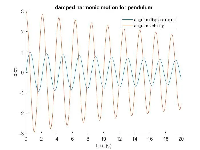
• Plotting the graph for angular dispacement and angular velocity with respect to time using plot command and proving suitable legends using title command.

The graph for angular dispacement and angular velocity with respect to time is as shown below

• Using a counter variable requred for counting the step will be taken for capturing the plots of angulur movement of simple pedulum.
• Using loop command for creating each plot for simple pendulum for satisfying the given condition for its angular movemnet.
• Creating animation for simple pendulum, for this first creating plots for pendulm string and bob
• using plot command by specifying start and end position along x and y axis, also specifying proper linewidth for line and string. specifying the bob properties like size and colour by using markersize and markerFacecolor commands.
• Caputuring each the plots for each movement for penulum using getframe command for creating animation and taking M as as array varible for stroing all captured frame.
• Using the end command for ending the for loop.
• Creating a movie of all captured frame stored in variable M by using Movie(M) command.
• Creating video file in .avi format under videofile variable using a function VideoWriter command.
• Opening a videofile for playing the video using open(videofile) command.
• Finally writing a videofile using writeVideo(videofile,M) command for saving video of the disk and closing the video by using close(vdeofile) command.
• The animation video for the simple pednulum can be seen by the link:

https://www.youtube.com/watch?v=1XveSCbFabE

Error Faced in program and solved:

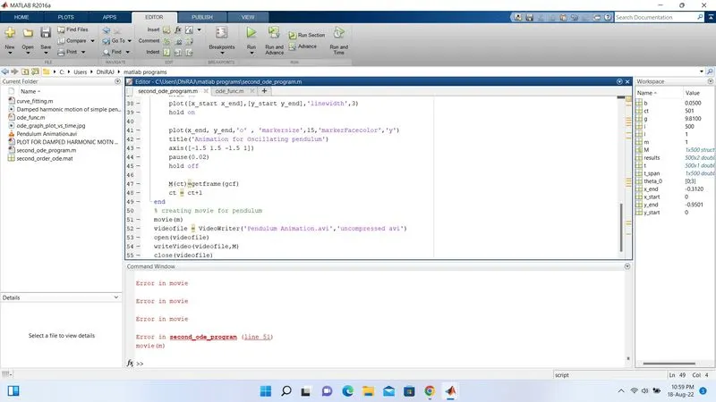
An error ocurred while running a programm for creating and playing the completeing animation video for simple pedulum due which it fails to play the complete video and saving it to the disk. This error was ocurred due to taking wrong variable for the movie function which was then corrected from "m" to "M" and problem solved.