Project 2 - Rankine cycle Simulator

Rankine Cycle Simulator in MATLAB

Aim: To create Rankine cycle simulator in MATLAB based on user input

Objectives:

• To calculate state points of Rankine cycle based on user input.
• To plot T-S and H-S plots for given set of inputs.
• To write a report on working of Rankine cycle simulator.

Given Data:

• Turbine Inlet Temperature = 400 ^OC.
• Turbine Inlet pressure = 30 bars.
• Turbine Outlet pressure = 0.05 bar = Condenser Inlet pressure.
• The standard Xsteam library to get the steam table data for water.

Solution:

Theory

The Rankine cycle system consists of a pump, boiler, turbine, and condenser. The pump delivers liquid water to the boiler. The boiler heated by the solar heat converts water to superheated steam. This steam is used to run the turbine which powers the generator. Steam leaves the turbine and becomes cooled to liquid state in the condenser. Then the liquid is pressurized by the pump and goes back to the boiler. And the cycle continues. Schematically, this process is represented in below Figure.

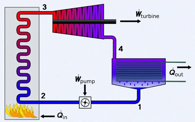
Figure (1)

In an ideal Rankine cycle, all the units operate with the steady-state flow, and the kinetic and potential energy of the fluid are considered to be negligible compared to the temperature and pressure effects.

The work terms for each component of the cycle can be expressed as follows.

The work done by the pump to compress water (W_pump) can be represented as the change in enthalpy (H) of the water (fluid) before entering the pump and after leaving the pump:

Wpump=H2−H1

In this case, we assume there is no heat exchange with the surroundings, so the energy is not lost (which is an ideal scenario). The process, which is not accompanied by any heat exchange with the environment, is termed "adiabatic." So, this step 1-2 is adiabatic compression.

The next process 2-3 takes place in the boiler. The energy balance in the boiler can be expressed as the change in enthalpy of the fluid from the "before" state (compressed liquid) to "after" state (superheated steam):

Qin=H3−H2

Where Q_in is the heat used by the boiler. This heat is supplied to the boiler from the solar concentrator. There is no pressure change in the boiler, only heat transfer to the fluid; therefore, no mechanical work is done here.

The next process 3-4 is expansion of the steam in the turbine. The work done through that process is the useful work, which is the main purpose of the cycle:

Wturbine=H3−H

Here, we again assume that there is no heat exchange with the surrounding, so all the fluid energy change is converted to work. Note that the enthalpy change is written as "before" minus "after" because the energy of the superheated compressed steam is higher than the expanded steam after it exits the turbine. So, this expression gives us the positive work value.

Lastly, the process 4-1 is steam cooling and condensation. The energy balance on the condenser will be:

Qout=H4−H1

At this stage, the extra heat is withdrawn from the system, and water returns to liquid state. This is important for the Rankine cycle from technological standpoint, since pumps employed in the system require liquid medium to work efficiently and may have problems with water-vapor mixtures.

The energy balance for the whole cycle is then can be expressed via the following equation:

(Qin−Qout) −(Wturbine−Wpump) =0

The net work done by the system is W_turbine-W_pump. Therefore, the thermal efficiency of this cycle can be presented as follows:

η = Wnet / Qin = 1 – Qout / Qin

The basic Rankine cycle is presented in terms of temperature and entropy change in following Figure . The ideal state of this cycle is reflected in the vertical lines 1-2 and 3-4, when the fluid compressed and expanded. Those processes are shown to proceed isentropically, i.e., without entropy change. That rarely happens in real life. Some fluid friction losses and dissipation of some heat to the surrounding usually makes this system deviate from the ideality (as for example, shown by the dashed lines).

In a non-ideal cycle, fluid friction results in the lower pressure in the line. To compensate for this pressure, drop the water needs to be pumped to a higher pressure. Heat loss can happen when steam flows through the connecting pipes and the cycle components, which are not perfectly insulated. To maintain the same work output, more heat needs to be transferred to the steam in the boiler.

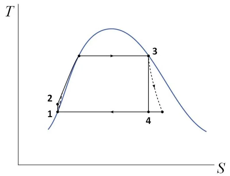
Figure (2)

Varieties of the Rankine Cycle

There are several scenarios of employment of the Rankine steam cycle in power plants, including solar plants. Those scenarios intend to increase the overall efficiency of the system.

There are three ways to increase the efficiency of the basic Rankine cycle:

1. Decreasing condenser pressure. This results in lower heat rejection temperature of the fluid in the condenser (pushing point 4 on the diagram in Fig. 2 downward), thus allowing the system to produce greater net work.
2. Superheating steam to a higher temperature allows achieving higher temperature differential, thus increasing the amount of work done by the cycle.
3. Increasing the boiler pressure results in higher average steam temperature in the boiler. This effect allows additional work to be done in phase 2-3 (Fig. 3c). However, there is some loss of useful work in phase 3-4 because of necessity to re-heat the steam. Reheating is used to mitigate higher moisture content of the high-pressure steam.

The above-described efficiency modifications are illustrated in Figure (c).

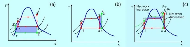
Figure (3)

Figure (3). Effects of different parameters on the work output of the Rankine cycle:

(a). Effect of decreasing condenser's pressure,

(b). Effect of superheating steam to a higher temperature,

(c). effect of increasing boiler pressure.

The shaded area shows the extra work performed by the system due to each parameter change.

The red curve corresponds to the basic cycle, and green curve shows the adjusted cycle.

Another variety of Rankine cycle is the Regenerative Rankine. The idea behind the regenerative cycle is to increase the temperature of the feed water that is supplied to the boiler. Why is it desirable? Higher water temperature would allow some energy savings for steam generation. So, some of the steam that exits the turbine is used for pre-heating the feed water for the boiler. This process is called regeneration. Heat transfer can be achieved using a heat exchanger (regenerator). There are two types of feed water heaters: open and closed.

The open feed water heater is essentially a mixing chamber, where the steam extracted from turbine is combined with water from the pump. The fluid that exits the mixing chamber is saturated water. The closed feed water heater is a heat exchanger, inside which the steam condenses on the outside of the tube carrying the feed water. As a result, the feed water temperature is increased. The pressures of the steam and the feed water do not need to be matched since the flows are not mixing. Without heat regeneration, the feed water temperature would be much lower and would require more energy from the heat source for the boiler. Regeneration helps raise the overall efficiency of the system.

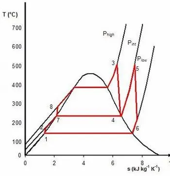
Figure (4)

Figure (4), T-S diagram of the regenerative Rankine cycle. In case of open feed water-heater, the phase 2-7 corresponds to the mixing, and 7-8 is the second compression of the fluid before the boiler.

Stepwise Explanation of code with comments:

% Rankine Cycle Simulator
clear all % Clearing all the window
close all % cloasing all output windows
clc % clearing command window

% Printing Introduction of Rankine cycle process
fprintf('RANKINE CYCLE SIMULATOR \n')
fprintf('1-2 is isentropic expansion in the Turbine \n')
fprintf('2-3 is Constant Pressure Heat Rejection by the Condenser \n')
fprintf('3-4 is isentropic Compression in pump \n')
fprintf('4-1 is Constant Pressure Heat Addition by the Boiler \n')

% Taking Inputs from User 
P1 = input('Enter the Pressure at the Turbine Inlet (in bar):'); % Taking input inlet pressure of turbine
T1 = input('Enter the Temprature at the Turbine Inlet (in Degree Celcius): '); % Taking input inlet temperature
P2 = input('Enter the Pressure at the Turbine Outlet (in bar): '); % Taking input outlet pressure of turbine

% State point 1
H1 = XSteam('h_pt',P1,T1);  % Enthalpy at point 1
S1 = XSteam('s_pt',P1,T1);  % Entropy at point 1
Hf1 = XSteam('hL_p',P1);    % Enthalpy of saturated liquid at point 1
Hg1 = XSteam('hV_p',P1);    % Enthaply of saturated vapour at point 1
Ts1 = XSteam('Tsat_p',P1);  % Saturation Temprature at point 1
Sf1 = XSteam('sL_p',P1);    % Entropy of saturated liquid at point 1
Sg1 = XSteam('sV_p',P1);    % Entropy of saturated vapour at point 1

% State point 2
S2 = S1; % entropy is conctant at point 1 and 2
Sf2 = XSteam('sL_p',P2); % Entropy of saturated liquid at point 2
Sg2 = XSteam('sV_p',P2); % Entropy of saturated vapour at point 2
x = (S2-Sf2)/(Sg2-Sf2);  % Dryness fraction at point 2
Hf2 = XSteam('hL_p',P2); % Enthalpy of saturated liquid at point 2
Hg2 = XSteam('hV_p',P2); % Enthaply of saturated vapour at point 2
H2 = Hf2 + x*(Hg2-Hf2);  % Enthalpy at point 2
T2 = XSteam('T_ph',P2,H2); % Temprature at point 2
Ts2 = XSteam('Tsat_p',P2); % Saturated Temprature at point 2

% State point 3
H3 = Hf2; % Enthalpy at pint 3 is same as enthalpy of saturated liquid at point 2
S3 = Sf2; % Entropy at pint 3 is same as entropy of saturated liquid at point 2
T3 = T2; % Temperature is same at point 2 and 3
P3 = P2; % Pressure is constant at point 2 and 3

% State point 4
P4 = P1; % pressure is constant at point 4 and 1
S4 = S3; % Entropy is constant at point 3 and 4
H4 = XSteam('h_ps',P4,S4); % Enthaly at point 4
T4 = XSteam('T_ps',P4,S4); % Temperature at point 4

t = linspace(0,374,500);    % temp space for plotting saturation cutves

%Plot T-S Diagram
figure(1) % Creating window1 for plot
hold on % holding the plot window

% Plot Saturation Curve
for i = 1 : length(t) % using for loop upto timespan
   plot(XSteam('sL_T',t(i)),t(i),'.','color','b') % plotting Entropy of saturated liduid at contant temperature
   plot(XSteam('sV_T',t(i)),t(i),'.','color','b') % plotting Entropy of saturated vapour at contant temperature
end % ending the for loop

% Plot Cycle
plot([S1 S2],[T1 T2],'linewidth',2,'color','r') % plotting entropy and temperature at point 1 and 2
if x>1  % applying condition for dryness fraction
    T3 = Ts2; % if true then saturated temperature at point 2 will be same to teperature at point 3
    plot([S2 Sg2 S3 S4],[T2 Ts2 T3 T4],'linewidth',2,'color','r') % plotting entropy and temperature at point 2 and 3
    T2 = Ts2; % saturated temperature at point 2 will be same to teperature at point 2
else
    plot([S2 S3 S4],[T2 T3 T4],'linewidth',2,'color','r') % if false the plot entropy vs. temperature at point 2, 3 and 4
end % ending the condition

l = linspace(T1,T2,1000); % initilizing temperature 1 to 2 
for i = 1 : length(l) % using for loop upto lentgh value
    plot(XSteam('s_pT',P1,l(i)),l(i),'.','color','r') % plotting entropy at constant pressure and temperature
end % ending for loop

plot([Sf1 Sg1],[Ts1 Ts1],'linewidth',2,'color','r') % plotting entropy of saturated liquid and vapour vs. saturated temperature at point 1
xlabel('Entropy[KJ/Kg-K]') % labeling x-axis as entropy 
ylabel('Temprature[K]') % labeling y-axis as temperature
title('T-S Diagram') % Entitling the the plot 

% Plot H-S Diagram
figure(2) % creating window2
hold on % holding window

% Plot Saturation Curve
for i = 1 : length(t) % using for loop upto length(t)
    plot(XSteam('sL_T',t(i)),XSteam('hL_T',t(i)),'.','color','b') % Plotting entropy of saturated liquid at constant temperature
    plot(XSteam('sV_T',t(i)),XSteam('hV_T',t(i)),'.','color','b') % Plotting entropy of saturated vapour at constant temperature
end % ending for loop

% Plot Cycle
plot([S1 S2 S3 S4 S1],[H1 H2 H3 H4 H1],'linewidth',2,'color','r')% plotting entropy vs enthalpy at point 1,2,3 and 4
xlabel('Entropy[KJ/Kg-K]') % Labeling x-axis as entropy
ylabel('Enthalpy[KJ/Kg]') % Labeling y-axis as enthalpy
title('H-S Diagram') % entitling the plot as H-S diagram

% performing calculations

Wt = H1-H2; % calculating Turbine Work at constant temperature
Wp = H4-H3; % calculating Pump Work at constant temperature

Qin = H1-H4; % Calutaing Heat Addition
Qout = H2-H3; % Calculating Heat Rejection

Wnet = Wt-Wp; % Calculating Net Work
Ntherm = (Wnet/Qin)*100; % Calculating Thermal Efficiency

SSC = 3600/Wnet; % calculating Specific steam consumption


BWR = Wp/Wt; % Calculating Back Work Ratio

% Print Results
fprintf('\n Results \n')
fprintf('At State Point 1:\n')
fprintf('P1 is : %.2f bar \n',P1)
fprintf('T1 is : %.2f Deg Celcius \n',T1)
fprintf('H1 is : %.2f KJ/Kg \n',H1)
fprintf('S1 is : %.2f KJ/Kg-K \n',S1)

fprintf('\n At State Point 2:\n')
fprintf('P2 is : %.2f bar \n',P2)
fprintf('T2 is : %.2f Deg Celcius \n',T2)
fprintf('H2 is : %.2f KJ/Kg \n',H2)
fprintf('S2 is : %.2f KJ/Kg-K \n',S2)

fprintf('\n At State Point 3: \n')
fprintf('P3 is : %.2f bar \n',P3)
fprintf('T3 is : %.2f Deg Celcius \n',T3)
fprintf('H3 is : %.2f KJ/Kg \n',H3)
fprintf('S3 is : %.2f KJ/Kg-K \n',S3)

fprintf('\n At State Point 4: \n')
fprintf('P4 is : %.2f bar \n',P4)
fprintf('T4 is : %.2f Deg Celcius \n',T4)
fprintf('H4 is : %.2f KJ/Kg \n',H4)
fprintf('S4 is : %.2f KJ/Kg-K \n',S4)

fprintf('\n Wt is : %.2f KJ/Kg \n',Wt)
fprintf('Wp is : %.2f KJ/Kg \n',Wp)
fprintf('Wnet is : %.2f KJ/Kg \n',Wnet)
fprintf('Thermal Efficiency is : %.2f percent \n',Ntherm)
fprintf('S.S.C. is : %.2f Kg/KWh \n',SSC) 
fprintf('Back Work Ratio is : %.3f \n',BWR)

Output:

Command windows

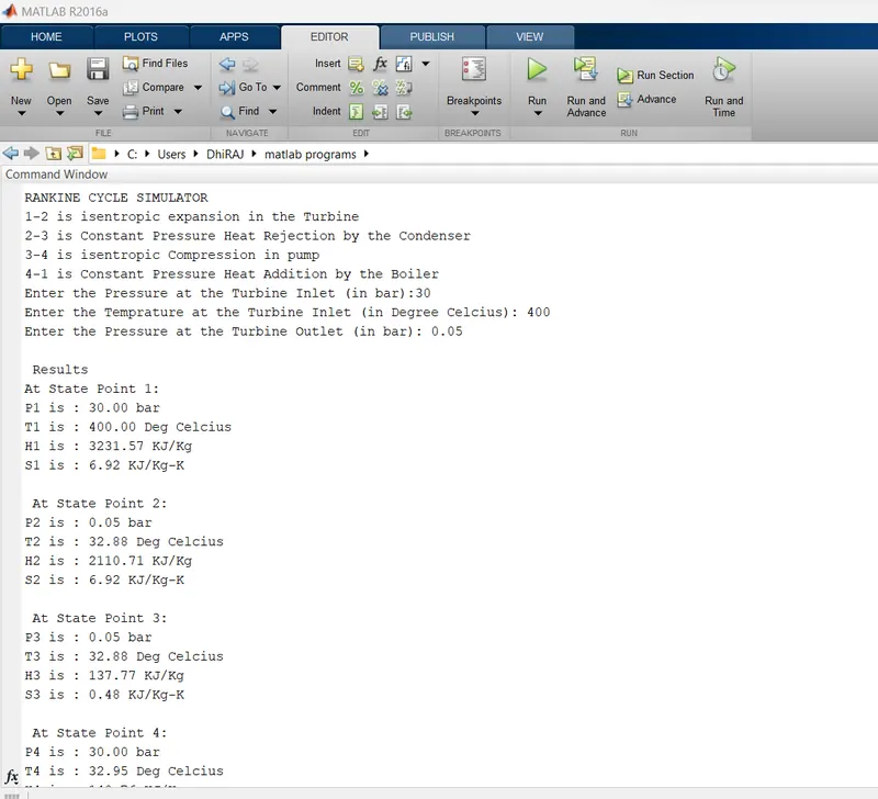
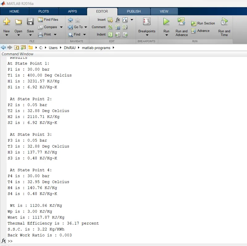
Workspace

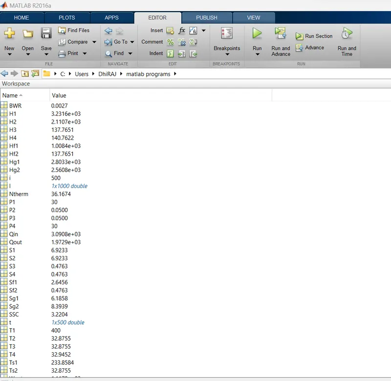
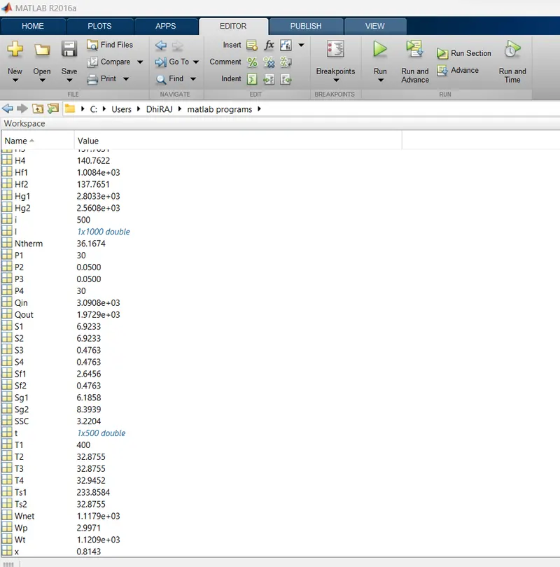
Errors faced while programming:

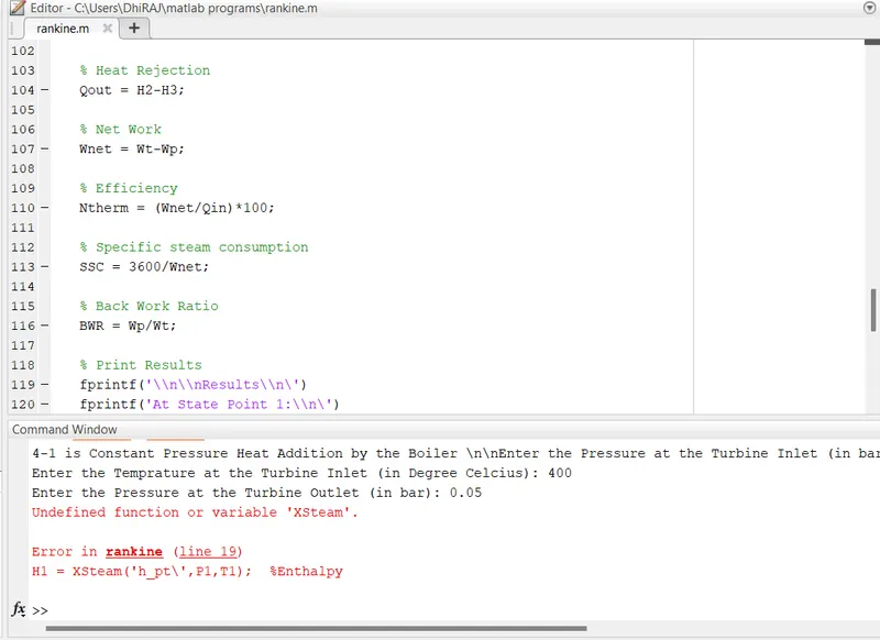
1. Error ocurred while running program in line 19 showed un-identified fuction or variable 'Xsteam' as shown in below snapshot. The error removed by removing the symbol backlash (\)

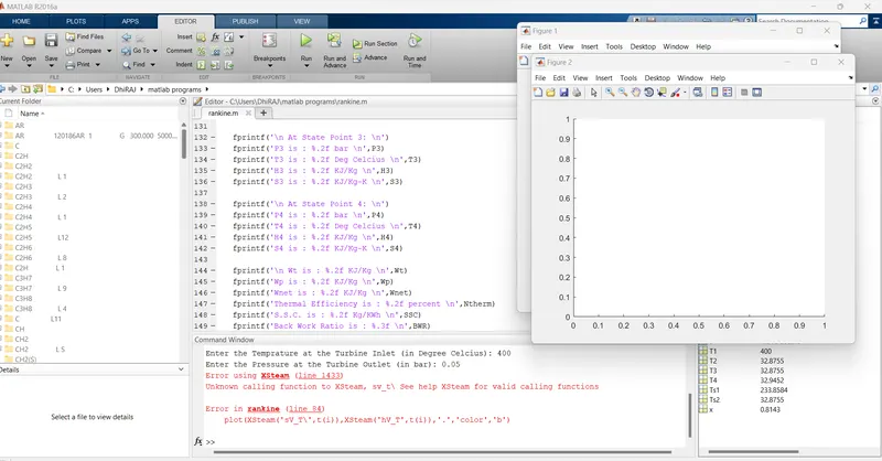
2. The same error ocurred due to same problem as shown in snapshot and corrected by removing backlash (\) symbol.

Conclusion:

• The state points of the Rankine Cycle are calculated by using the steam table data for water from standard MATLAB Xsteam library.
• Programs are written in MATLAB to compute property values of water at three regions and then employed by another program which will simulate a Rankine cycle.
• Plots for T-s, h-s and p-v plots of the Rankine Cycle are plotted and the work and efficiency of the Rankine Cycle are calculated.

References:

7.6. Rankine cycle | EME 812: Utility Solar Power and Concentration (psu.edu)

Rankine cycle - Wikipedia

RANKINE CYCLE (thermopedia.com)