Week 4.1 - Solving second order ODEs

Solution:- Here we need to calcultate the ordinary differential equation and simulate the pendulum as per its transient behaviour.

Objective: - write a program that solves the following 2nd order ODE. This ODE represents the equation of motion of a simple pendulum with damping coefficient is 0.05 and simulate using MATLAB code

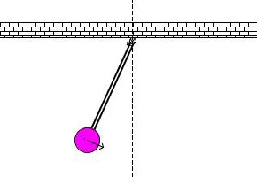
Theory:- Simple Pendulum: - A pendulum is a weight suspended from a pivot so that it can swing freely. When a pendulum is displaced sideways from its resting, equilibrium position, it is subject to a restoring force due to gravity that will accelerate it back toward the equilibrium position.

Working of Simple Pendulum:- A simple pendulum consists of a mass m hanging at the end of a string of length L. The
period of a pendulum or any oscillatory motion is the time required for one complete
cycle, that is, the time to go back and forth once.

Here the derrived 2nd order ordinary differential equation

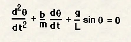
In this given equation here,

g = gravity in m/s2,

L = length of the pendulum in m,

m = mass of the ball in kg,

b=damping coefficient.

What we need to Implement:-

Here we need to write a program in Matlab that will simulate the pendulum motion use,

L=1 meter,

m=1 kg,

b=0.05.

g=9.81 m/s2.

Simulate the motion between 0-20 sec, for angular displacement=0, angular velocity=3 rad/sec at time t=0. And we need to use this information to animate the motion of the pendulum, as shown in the below figure.

Ordinary Differential Equation:-

A differential equation containing one or more function of independent variable is said to be ordinary differential equation.

Uses of Ordinary Differential equation:-

• Used in the study of changes where it helps in analyses the dynamic problems involving flow studies, and behavioral studies.
• It also helps in computational solutions of real world problems.
• Highly used in fluid dynamics, structural analysis, and thermal studies.

Step Wise Explanation of the code:-

• 1^st we initialize the input variables like L, m, b, g.
• Create time span using linspace command that is 0-20 sec and 500 values between it.
• Initial condition theta is defined that create row and column vector.
• Now solving the equations using ode45 function and created function ode_func.
• Now plotting the transient behavior of pendulum.
• Define axis and named the x and y label.
• Plotting various figures like fixed junction for hanging the pendulum.
• Plotting thread and ball of pendulum using linewidth and marker comand
• Now creating the movie animation using videowrite command of various test figures.

Errors that we faced during writing the code for ode function.

figure(2) % Creating figure window for plotting an animation of pendulum

  hold on   % hold the figure window 2

  plot([-1 1],[1 1],'linewidth',8);     % Plotting fixed roof for pendulum's fixed point

  plot([x0 x1],[y0 y1],'linewidth',3);  % Plotting link or thred by which pendulum's ball is held

  plot(x1, y1, 'Marker','o','Markersize',30,'Markerfacecolor','b');  % Plotting the ball of pendulum

  plot(x0, y0,'Marker','o','Markersize', 9,'Markerfacecolor',[1 1 1]);  % Plotting the fixed point of       pendulum

  line([x0 x0],[y0 -1.8],'linestyle','--','color','r','linewidth',3); % Plotting of center line 

  axis(‘Tight’);   % To adjust axis as our requirements

  pause(0.03); % update the figure at interval of 0.03

  grid on % Make the grid visible

  text = sprintf('test%d.png',ct); % Create png file for each image created by plotting

  M(ct)=getframe(gcf);  % Capturing the current plot for combining the later

  clf();   % Clearing the current graphic image

  ct=ct+1; % Increment in figure counter

end        % end for loop

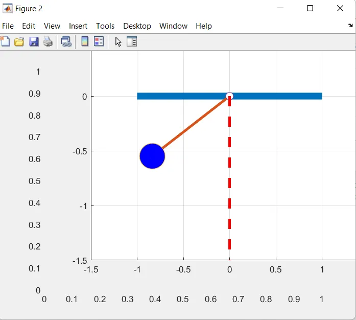
While plotting the axis for this we made a mistake and we get output like this:-

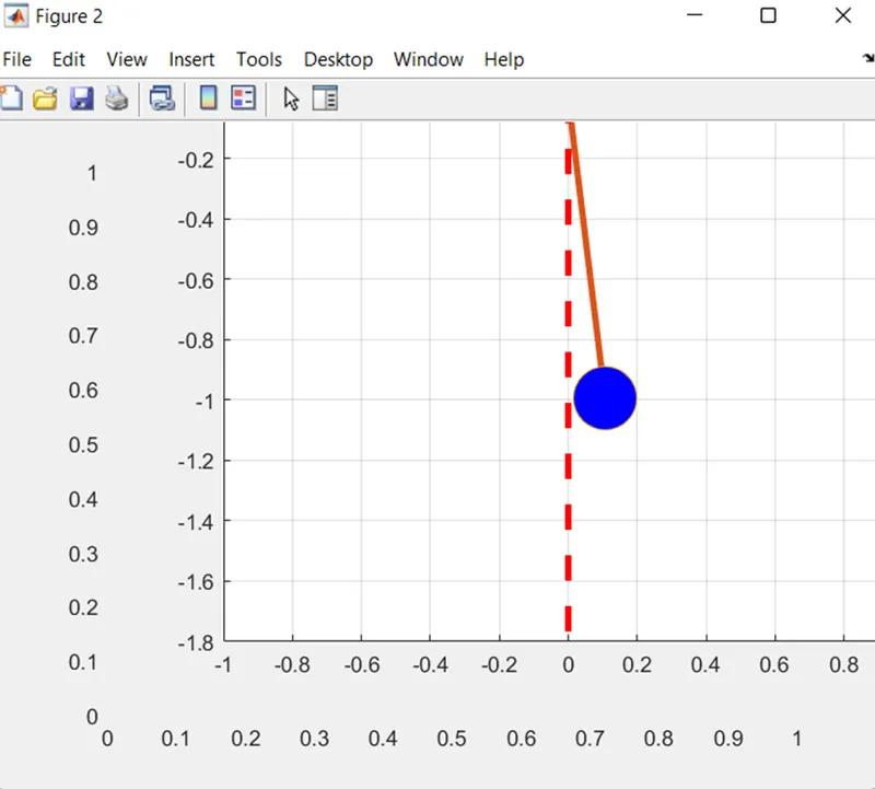
Figure 2:-

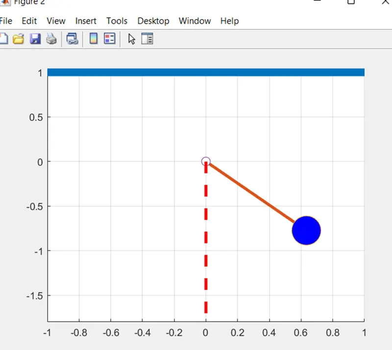
How to overcome this Error

After analyzing the plot and axis we get to know that where are we missing the things then we correct it accordingly.

figure(2) % Creating figure window for plotting an animation of pendulum

hold on   % hold the figure window 2

plot([-1 1],[0 0],'linewidth',8);     % Plotting fixed roof for pendulum's fixed point

plot([x0 x1],[y0 y1],'linewidth',3);  % Plotting link or thread by which pendulum's ball is stiched

plot(x1, y1, 'Marker','o','Markersize',30,'Markerfacecolor','b');  % Plotting the ball of pendulum

plot(x0, y0,'Marker','o','Markersize', 9,'Markerfacecolor',[1 1 1]);  % Plotting the fixed point of pendulum

line([x0 x0],[y0 -1.8],'linestyle','--','color','r','linewidth',3); % Plotting of center line 

axis([-1.5 1.5 -1.5 0.5]);   % To adjust axis as our requirements

pause(0.03); % update the figure at interval of 0.03

grid on % Make the grid visible

text = sprintf('test%d.png',ct); % Create png file for each image created by plotting

M(ct)=getframe(gcf);  % Capturing the current plot for combining the later

clf();   % Clearing the current graphic image

ct=ct+1; % Increment in figure counter

 

Now Final Code:-

# Main and Driver code for the simulation of pendulum:-

ct=1; % Assign value 1 to counter
for i=1:length(results(:,1)) % Assign value to i 
  
  % Origin or starting position of pendulum which is fixed
  x0=0;
  y0=0;
  % Varied value for end point of pendulum
  x1=L*sin(results(i,1));
  y1=-L*cos(results(i,1));
  
  figure(2) % Creating figure window for plotting an animation of pendulum 
  hold on   % hold the figure window 2
  plot([-1 1],[0 0],'linewidth',8);     % Plotting fixed roof for pendulum's fixed point
  plot([x0 x1],[y0 y1],'linewidth',3);  % Plotting link or thread by which pendulum's ball is stiched
  plot(x1, y1, 'Marker','o','Markersize',30,'Markerfacecolor','b');  % Plotting the ball of pendulum
  plot(x0, y0,'Marker','o','Markersize', 9,'Markerfacecolor',[1 1 1]);  % Plotting the fixed point of pendulum
  line([x0 x0],[y0 -1.8],'linestyle','--','color','r','linewidth',3); % Plotting of center line  
  axis([-1.5 1.5 -1.5 0.5]);   % To adjust axis as our requirements
  pause(0.03); % update the figure at interval of 0.03
  grid on % Make the grid visible 
  text = sprintf('test%d.png',ct); % Create png file for each image created by plotting
  M(ct)=getframe(gcf);  % Capturing the current plot for combining the later
  clf();   % Clearing the current graphic image
  ct=ct+1; % Increment in figure counter

end        % end of for loop

movie(M);           % Making the movie from collected FRAME
% A video file is created of avi type to save animation
videofile=VideoWriter('Motion_Of_pendulam.avi','Uncompressed AVI');
open(videofile);    % opening of videofile 
writeVideo(videofile,M);% writing the movie in the created video file
close(videofile);   % video file is closed

# Function code to calculate the Ordinary Differential equation:-

function [dtheta_dt]= ode_func(t, theta, b, m, g, L)
theta1=theta(1)
theta2=theta(2)
dtheta1_dt=theta2;
dtheta2_dt=-(b/m)*theta2 -(g/L)*sin(theta1);
dtheta_dt=[dtheta1_dt; dtheta2_dt];
end

# Final Output that we get after correcting the code:-

Here in this figure its showing the damping of the pendulum that means displacement w.r.t time:-

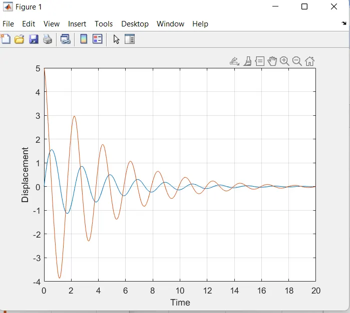
Here in this figure its showing how the displacement of pendulum takes place.

Here video link of youtube for the simulation:-

https://youtu.be/jIo53T47u-4

Simulation :-