Week 4.1 - Solving second order ODEs

AIM : To solve the second order derivative of the quadratic equation.

`(d^2theta)/(dt^2)+b/m(d theta)/(dt)+(g/l)sin(theta)=0`

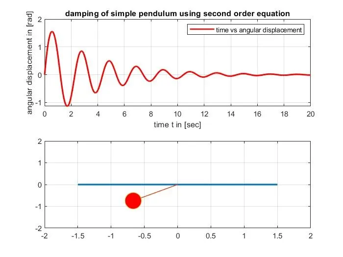
THEORY = In this we solve the above shown quadratic equation using an inbuilt solver in matlab itself.while solving this we uses the ode45 as the solver which is used for only solving linear equation so intially be simplify the quadratic equation into a linear equation by various substitution and then solve it then we plot the various poits of the pendulum and with those graphs we create a video file and then we get the movement of the pendulum.

function[dtheta_dt] = ode_func(t,theta,b,g,l,m)    
    theta1 = theta(1);
    theta2 = theta(2);
    dtheta1_dt = theta2;
    dtheta2_dt = -(b/m)*theta2-(g/l)*sin(theta1);
    dtheta_dt = [dtheta1_dt;dtheta2_dt];
end

clear all
close all
clc

% input variable
b = 0.05;  %  damping coe 
g = 9.81;  % aceeg in  'm/s2
l = 1;         % length in  'm'
m = 0.1;  % mass in 'kg'

%intial conditions
theta_0 = [0;5];  % 0 angular sdisp in 'rad/s, 5= angular vel in 'rad/se2


%time points
t_span = linspace(0,20,500);  % simiutlion time (0 to 20) , taking graid 500

%solve ode
[t,results] = ode45(@(t,theta)ode_func(t,theta,b,g,l,m),t_span,theta_0);


%plotting
figure (1)
subplot(2,1,1)
plot(t,results(:,1),'color','r' ,'linewidth',1.5);
xlabel('time t in [sec]');
ylabel('angular displacement in [rad]');
legend('time vs angular displacement');  %legend
title ('damping of simple pendulum using second order equation');
grid on;
subplot(2,1,2)
plot(t,results(:,2),'color','g','linewidth',1.5);
xlabel('time t in sec');
ylabel('angular velocity[rad/sec]');
grid on;
legend('time vs angular velocity'); %legend

% animation of the simple pendulum,placing the 'fixed at a point'
figure(2) %showing another video of the image

ct = 1;
for i = 1:length(results(:,1))
      x0 = 0;
      y0 = 0;
      % using trignometric function
      x1 = 1*sin(results(i,1));
      y1 = -1*cos(results(i,1));
      %plotting the 'support rod' between (-0.5,0,0.5)
      plot([-1.5 1.5],[0 0],'linewidth',2);
      hold on
      plot([x0 x1],[y0 y1],'linewidth',1);
      plot(x1,y1,'o','markersize',20,'markerfacecolor','r');
      axis([-2 2 -2 2 ]) %label x axis (-2,2) and y axis (-2,2)
      grid on
      pause(0.03) %time pause
      M(ct) = getframe(gcf);% get current figure
      hold off
      ct = ct+1
end
movie(M) %movie file
videofile = VideoWriter('simple_pendulum.avi');%create video
open(videofile) %open video file


writeVideo(videofile,M); %capture the figure
close(videofile) %close the video

  

in this we start with the usual commands clear all, close all, clc, so that whatever codes or other programmes in the page gets

delected so that we get a fresh page.after this we define the variables such as b,g,l,m where b represents the damping coefficient,g represents the gravitational force,l represents the length of the connecting thread and m is the mass of the bob used.then we give the intial conditions the theta the number of divisions of the time.then we use another page named ode_func where we does various substitution and break down the quadratic equation into a linear equation so that we could use ode45 solver to plot the graph of time vs angular velocity and time vs angular displacement then we use the write video to create a video file where the video file is an animated video showin the movement of the to and fro motion of the pendulum.

CONCLUSION : so i was able to get the seconder derivative of the quadratic equation and also was able to create a videofile showing the movement of the pendulum.

https://drive.google.com/file/d/1TtA5FomCTIew-dsk6mk7vf0T6_Ob5NhC/view?usp=sharing