Week 4.1 - Solving second order ODEs

REPORT:

Aim: To simulate the transient behaviour of simple pendulum.

Objective: Objective is to write a program that solves the following ODE. This ODE represents the equation of motion of a simple pendulum with damping.

Governing equation: Second order ODE is

d²(theta)/dt² + b/m d(theta) /dt + g/l sin(theta) = 0

In the above equation,

g = gravity in m/s2,

L = length of the pendulum in m,

m = mass of the ball in kg,

b=damping coefficient.

Body of the Report:

Matlab software is used to get the required output.

Program:

1) ODE function:

function [dtheta_dt] = ode_func(t,theta,b,g,l,m)

theta1 = theta(1)
theta2 = theta(2)
dtheta1_dt = theta2;
dtheta2_dt = -(b/m)*theta2 - (g/l)*sin(theta1);
dtheta_dt =  [dtheta1_dt; dtheta2_dt];
end

2) Main program:

clear all
close all
clc

b = 0.05;
g = 9.81;
l = 1;
m = 1;

% initial condition
theta_0 = [0;3];

% time points
t_span = linspace(0,20,500);

% solve ode
[t, results] = ode45(@(t,theta) ode_func(t, theta, b,g,l,m),t_span, theta_0);

%plotting
figure(1)
plot(t,results(:,1))
hold on
plot(t,results(:,2))
title('for simple pendulum')
ylabel('angular velocity / displacement')
xlabel('time')
legend('displacement', 'angular velocity')

%animation of pendulum
amplitude=results(:,1);
%store amplitude values in seperate matrix for loop 
p=1;
for i=1:length(amplitude)
    angle=amplitude(i);
    figure(2)
    title('simple pendulum')

    %fix point of pendulum
    x0=0;
    y0=0;
    %cordinate of mass ball / another end of pendulum
    x1=l*sin(angle);
    y1=-l*cos(angle);

    %plot
    plot([-1.1 1.1,],[0 0], 'LineWidth',2); %celling line
    hold on 
    plot([x0 x1],[y0 y1],'color','g','LineWidth',2)%string
    plot(x1,y1, 'o','Markers',20,'MarkerFaceColor',[1 1 0])%mass ball
    hold off %removing previous position
    grid on
    axis([-1.5 1.5 -1.5 0.5])
    pause(0.001)
    M(p) = getframe(gcf);
    p = p+1;
end

movie(M)
videofile = VideoWriter('simple_pendulum.avi','Uncompressed AVI');
open(videofile)
writeVideo(videofile,M)
close(videofile)

Step wise explanation:

1. first step to solve higher order ODEs is to breaking down ODE in to series of first order ODEs. This has been done in the function program.
2. Then the main program is started with 'clear all', 'close all' and 'clc' command to clear all the previous variables in workspace, previous plots and command window respectively.
3. Then the inputs, initial conditions and the time span are inputed.
4. ODE solver is inputed and ODE function is introduced.
5. Graphs are listed for simple pendulum by inputing the cordinates of starting point of string of pendulum and the cordinates of ball/end point of pendulum string using for loop syntax.
6. contours are added in the form of P for pause of 0.001 sec.
7. for loop is ended
8. movie is created using the command videofile. in that the videofile is opend then its been written and then videofile is closed.
9. then the generated movie is saved as AVI file.

Link to see generated movie:

https://youtu.be/RzgQETnWzcY

Graph:

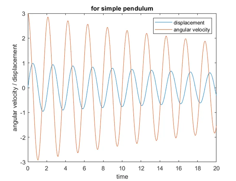
Conclusion: Thus the MATLAB program is written and the transient behavior of simple pendulum is created using MATLAB.