Week 4.1 - Solving second order ODEs

Aim: To evaluate the motion of simple pendulum by solving ODE using MATLAB

Theory:

In Engineering, ODE is used to describe the transient behavior of a system. A simple example is a pendulum. The way the pendulum moves depends on the Newtons second law. When this law is written down, we get a second order Ordinary Differential Equation that describes the position of the "ball" w.r.t time.

Consider a pendulum with ball of mass m">mm attached to the end string of length L">LL with other end being fixed.

where,

θ = Angular Displacement

g = Gravitational Acceleration

t = time

b = Damping Coefficient

For solving ODE using MATLAB, higher order differential equations needs to converted into a set of single order differential equations.

A typical approach to solving higher-order ordinary differential equations is to convert them to systems of first-order differential equations, and then solve those systems.

ODE of damped pendulum is 2^nd order ordinary differential equations , so we have to convert it into first order ODE.

d2θdt2+bmdθdt+gLsinθ=0d2θdt2+bmdθdt+gLsin⁡θ=0

In the above equation,

g = gravity in m/s²,

L = length of the pendulum in m,

m = mass of the ball in kg,

b=damping coefficient.

A typical approach to solving higher-order ordinary differential equations is to convert them to systems of first-order differential equations, and then solve those systems.

ODE of damped pendulum is 2^nd order ordinary differential equations , so we have to convert it into first order ODE.

d2θdt2+bmdθdt+gLsinθ=0d2θdt2+bmdθdt+gLsin⁡θ=0

In the above equation,

g = gravity in m/s²,

L = length of the pendulum in m,

m = mass of the ball in kg,

b=damping coefficient.

A typical approach to solving higher-order ordinary differential equations is to convert them to systems of first-order differential equations, and then solve those systems.

ODE of damped pendulum is 2^nd order ordinary differential equations , so we have to convert it into first order ODE.

d2θdt2+bmdθdt+gLsinθ=0d2θdt2+bmdθdt+gLsin⁡θ=0

In the above equation,

g = gravity in m/s²,

L = length of the pendulum in m,

m = mass of the ball in kg,

b=damping coefficient.

θ=θ1θ=θ1 (equation 1)

From equation 1:

dθdt=dθ1dt=θ2(equation2)dθdt=dθ1dt=θ2(equation2)

d2θ1dt2=ddt(dθ1dt)=dθ2dt(equation3)d2θ1dt2=ddt(dθ1dt)=dθ2dt(equation3)

From equation number 2,3:

dθ1dt=θ2(equation4)dθ1dt=θ2(equation4)

d2θ1dt2+bmdθ1dt+gLsinθ=0d2θ1dt2+bmdθ1dt+gLsin⁡θ=0

dθ2dt+bmθ2+gLsinθ1=0dθ2dt+bmθ2+gLsin⁡θ1=0

so

dθ2dt=−bmθ2−gLsinθ1(equation5)dθ2dt=-bmθ2-gLsin⁡θ1(equation5)

From equation number 4 and 5:

Writing equation in matrix format

ddt[θ1θ2]=[θ2−bmθ2−g2sinθ1]

Given initial condition:

L=1 metre,

m=1 kg,

b=0.05.

g=9.81 m/s2s2

L, m, b & g represents length of pendulum, mass of bob, damping co-efficient & gravity.

Initial conditions:

angular displacement=0,angular velocity=3 rad/sec at time t=0.

analysis time 0-20sec

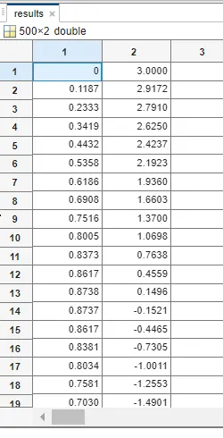
Below code will solve the ODE , will give the values of angular displacement and angular velocity for the given time slot and will plot the graphs of variaton of angular displacement vs time and variation of angular speed vs time.

MATLAB Main Program:

clear all
close all
clc

b=0.05;
g=9.81;
l=1;
m=0.1;

% initial condition
theta_0=[0;3];
% time points
t_span=linspace(0,20,500);

% solve ODE
[t,results]=ode45(@(t,theta) ode_func(t,theta,b,g,l,m),t_span, theta_0);
plot(t,results(:,1))
hold on
plot(t,results(:,2))
xlabel('time');
ylabel('Plot');
% creating animation
ct=1;
for i=1:500;

    x0=0;
    y0=0;
    x1=l*sin(results(i,1));
    y1=-1*cos(results(i,1));
    figure(2);
    plot([-1 1],[0 0],'LineWidth',10,'color','g');
    axis([-2 2 -2 2]);
    hold on
    line([x0 x1],[y0 y1],'linewidth',5,'color','b');
    plot(x1,y1,'o','markersize',25,'MarkerFaceColor','r');
    hold off
    M(ct)=getframe(gcf);
    ct=ct+1;
end
%creating movies
movie(M)
videofile=VideoWriter('ode_main.avi','Uncompressed AVI');
open(videofile);
 writeVideo(videofile,M)
close(videofile);


ode_function


function[dtheta_dt]=ode_func(t,theta,b,g,l,m)

theta1=theta(1);
theta2=theta(2);
dtheta1_dt=theta2;
dtheta2_dt=-(b/m)*theta2-(g/l)*sin(theta1);
dtheta_dt=[dtheta1_dt;dtheta2_dt];
end

ode_func converts second order differential equation into two single order differential equations.

Code is explained used comments at each section.

values of angular displacement and angular velocity for given time slot:

Response Curve:

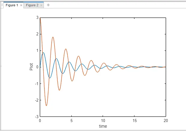
From above graph it can be observed that oscillation of pendulum are gradually damped as we can observe that angulalar displacement and angular velocity was gradually decreasing with time.

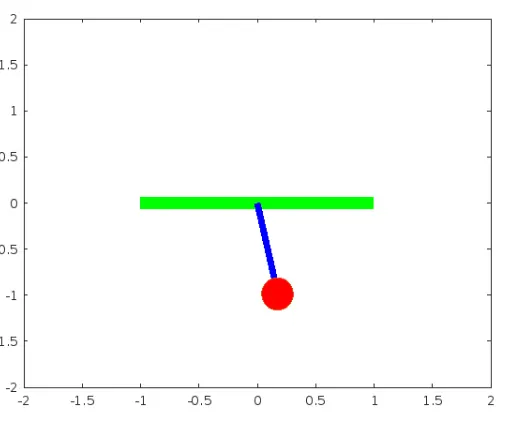
Animation:

Figure of animation plot-

Google drive link of animated plot:

https://youtu.be/JyeUltIKCk8

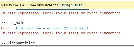
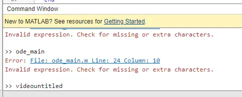
Error

i got the above error because the in my code i have taken xlabel(time); missing apostrophe after correctio i correct the missing

Conclusion:

1. ODE has been solved using ode45 in MATLAB
2. Motion of simple pendulum has been animated.
3. It was observed that as damping co-efficient increses ,motion of pendulum gets damped faster.