Week 4.1 - Solving Second-Order ODEs

Question

In Engineering, ODE is used to describe the transient behaviour of a system. A simple example is a pendulum

The way the pendulum moves depends on the Newton's second law. When this law is written down, we get a second-order Ordinary Differential Equation that describes the position of the "ball" w.r.t time.

Similarly, hundreds of ODEs describe key phenomena and if you can solve these equations, you can simulate any of these systems.

Your objective is to write a program that solves the following ODE. This ODE represents the equation of motion of a simple pendulum with damping.

`(d^2theta)/dt^2+(b/m)((d theta)/dt)+(g/L)sintheta =0`

In the above equation,

g = gravity in m/s2,

L = length of the pendulum in m,

m = mass of the ball in kg,

b=damping coefficient.

Write a program in Matlab\Octave that will simulate the pendulum motion,

use,

L=1 metre,

m=1 kg,

b=0.05.

g=9.81 m/s2.

Simulate the motion between 0-20 sec, for angular displacement=0, angular velocity=3 rad/sec at time t=0.

When you do this you will get the pendulum's position as a function of time. Use this information to animate the motion of the pendulum

Answers

Simple Pendulum

A simple pendulum is a mechanical arrangement that demonstrates periodic motion. It consists of a small bob of mass 'm' suspended in a thin string secured to a platform at its upper end of length 'L'. The simple pendulum is a mechanical system that sways or moves in an oscillatory motion. The motion occurs in a vertical plane driven by the gravitational force.

The motion of a simple pendulum can be described by the following second-order ordinary differential equation (ODE)

`(d^2theta)/dt^2+(g/L)sintheta =0`

Where g = Acceleration Due To Gravity = 9.81 m/sec

L = Length Of Pendulum

`theta`= Angular Displacement Of Pendulum

The following second-order differential equation can model the motion of a simple pendulum with damping.

`(d^2theta)/dt^2+(b/m)((d theta)/dt)+(g/L)sintheta =0`

Where b= Damping Coefficient

m= Mass Of Bob

To find the solution of these second-order ODEs, we need to split them into two first-order ODEs. This can be done by the following steps,

For a pendulum,

`(d^2theta)/dt^2+(b/m)((d theta)/dt)+(g/L)sintheta =0` ---------------------(1)

Take

`theta=theta1`

`(d theta)/dt = (d theta1)/dt = theta2` ---------------------(2)

`(d^2theta)/dt^2 = (d^2theta1)/dt^2 = d/dt((d theta1)/dt) = (d theta2)/dt` ---------------------(3)

(1) =>

`(d^2theta)/dt^2+(b/m)((d theta)/dt)+(g/L)sintheta =0`

`(d theta2)/dt + b/m.theta2 + g/L.sintheta1 = 0`

`(d theta2)/dt = -b/m.theta2 - g/L.sintheta1`

So, the second-order ODE is broken down into two sets of first-order ODEs

`(d theta)/dt = (d theta1)/dt = theta2` and `(d theta2)/dt = -b/m.theta2 - g/L.sintheta1`

The matrix representation for the above is given below.

`d/dt[[theta1],[theta2]] = [[theta2],[-b/mtheta2-g/Lsintheta1]]`

Function

Here we need to implement a function that solves an ODE. An ODE contains one independent variable and one or more of its derivatives concerning that variable. The function is named 'ODE_function' and it takes the values of t, theta, damping coefficient (b), acceleration due to gravity (g), length '(L)' and mass '(M)' of the pendulum. Here t and theta are the independent and dependent variables and the remaining values are constants to the ODE.

• Initially, we define the function with suitable input values. The input values include t, theta, damping coefficient (b), acceleration due to gravity (g), length '(L)' and mass '(M)' of the pendulum. Here t will be the independent variable and theta the dependent variable.
  
  
• theta1 and theta2 are computed from theta.
  
  
• Computing the first and second derivative of theta for t.
  
  
• Using these derivatives find the value dtheta_dt.
  
  
• End the function and save it as 'ODE_function'
  
  

% Starting the function initiation. The function has the following variables t, theta, b (damping coefficient), g (acceleration due to gravity), l (length of pendulum) and m (mass of bob)

function [dtheta_dt]= ODE_function(t,theta,b,g,l,m) 

% Computing the value of theta1 from theta
theta1=theta(1);

% Computing the value of theta2 from theta
theta2=theta(2);

% Computing the first derivative of theta for t
dtheta1_dt=theta2;

% Computing the second derivative of theta for t
dtheta2_dt=-(b/m)*theta2-(g/l)*sin(theta1);

% Computing the dtheta_dt using above derivatives 
dtheta_dt=[dtheta1_dt;dtheta2_dt];

% Ending the function
end

Matlab Code

• The code starts with creating the following variables. The Values are taken as user inputs. (Except g).
  b = Damping Coefficient
  g = Acceleration Due To Gravity = 9.81
  l = Length Of Pendulum
  m = Mass Of Bob
  
  
• Creating two arrays 'Theta_0 and T_Span' for storing the initial conditions and time points.
  
  
  
• Solving the ODE by using the function 'ode45' and 'ODE_function'. Store the values in an array.
  
  
  
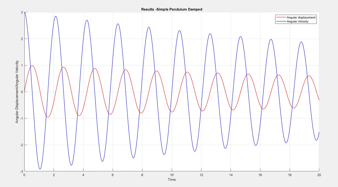
• From the values obtained by solving the ODE, plot the graphs of angular displacement and angular velocity with time within the same figure. Manage the plots by adding specifications and details.
  
  
• Create variable 'F', to represent the total number of frames and initially set the value of 'F' =1.
  
  
  
• Initiate the for loop.
  
  
• Assign the coordinate of the pendulum
  
  
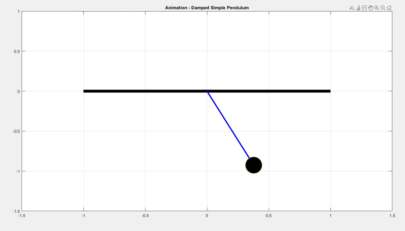
• Plot the simple pendulum by giving proper dimensions and coordinates. Manage them by adding specifications.
  
  
• Manage the plot
  
  
• Using the 'movie' command, play the sequence of frames stored in the structure 'M'.
  
  
• Using the 'videowriter' command, create a video with the sequence of frames, name the file 'Simple_Pendulum_Damped.avi' and store it in an animation file named 'Animation'.
  
  
• Using the 'open' command, open the animation file.
  
  
  
• Using the 'writevideo' command, write a video by combining both the animation file 'Animation' and the structure 'M'.
  
  
  
• Using the 'close' command, close the animation 'Animation'.
  

After that, the file will be saved and opened in Matlab. We can inspect the motion and trajectory of the bob using the animation

The Matlab code is attached below,

clear
close
clc


% Assigning Values For The Suitable Variables
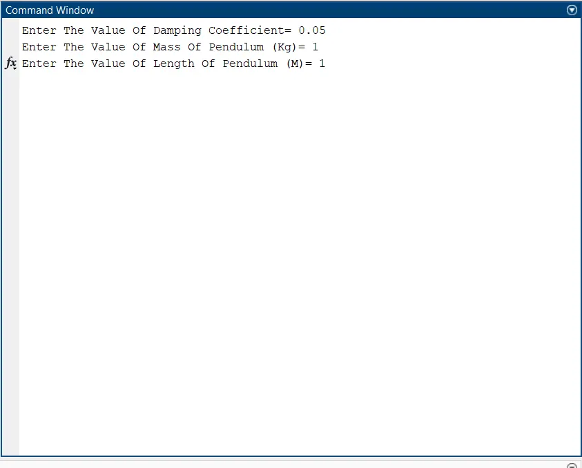
b= input('Enter The Value Of Damping Coefficient= ');
g= 9.81;
m= input('Enter The Value Of Mass Of Pendulum (Kg)= ');
L= input('Enter The Value Of Length Of Pendulum (M)= ');

% Creating An Array For Storing Initial Conditions
Theta_0 = [0;3];

% Array For The Time Points
T_span = linspace(0,20,500);

% Solving The ODE
[T,Results] = ode45(@(t,theta) ODE_function(t, theta, b,g,L,m), T_span, Theta_0);

% Plotting Graphs
figure(1)
hold on

% First Plot, T vs All Values In Column 1 of Result 
plot(T,Results(:,1),LineWidth=1,Color='red')

% Second Plot, T vs All Values In Column 2 of Result 
plot(T,Results(:,2),LineWidth=1,Color='blue')

% Labelling X-axis And Y-axis
xlabel('Time')
ylabel('Angular Displacement/Angular Velocity')

% Titling
title('esults -Simple Pendulum Damped')

% Grid Setting
grid on

% Setting Legend
legend('Angular displacement', 'Angular velocity')

% Create A Variable For Representing The Number Of Frames/Plots.  
F =1;

% For Loop Initiation
for i = 1:length(Results(:,1))

    % Assiging The Coordinates Of Pendulum 
    X0 = 0;     
    Y0 = 0;
    X1 = L*sin(Results(i,1));
    Y1 = -L*cos(Results(i,1));
 
    % Plotting Simple Pendulum
    figure(2)

    % Plotting The Base Line Which Simple Pendulum is Mounted
    plot([-1 1], [0 0], 'linewidth', 7,'Color','black')
    hold on

    % Plotting The String Of Pendulum
    plot([X0 X1],[Y0 Y1],'linewidth',3,Color='blue')
    hold on
 
    % Plotting The Bob
    plot(X1,Y1,'o','markersize',40,'markerFacecolor','black')
    
    % Grid Setting
    grid on

    % Titiling
    title('Animation - Damped Simple Pendulum')

    % Setting The Axes
    axis([-1.5 1.5 -1.5 1])
    pause(0.03)
    hold off

    % Creating A Structure To Store Every Frame Corresponding To The Value Of F
    M(F) = getframe(gcf);
    F = F+1;

 % Ending FOR Loop
 end
 
 
% Playing The Sequence Of Frames Stored In The Structure M
movie(M)

% Creating A Video With The Sequence Of Frames And Naming The File. Stored The Video File It In An Animation File  
Animation=VideoWriter('Simple_Pendulum_Damped.AVI','Uncompressed AVI');

% Opening The Animation Variable
open(Animation)

% Writing Video By Animation And The Frames Stored In Structure M
writeVideo(Animation,M)

% Closing The Animation 
close(Animation)

The results for the following values are given below,

L=1 metre,

m=1 kg,

b=0.05.

g=9.81 m/s2.

The drive link for the animation file is attached below.

https://drive.google.com/file/d/1o9zmsg6lBcNzHZL-S7hg9u-z996LGnEb/view?usp=sharing

Error Faced During The Matlab Code Development

• Hopefully, there are no major errors present during the code development. Some errors occurred due to the mistakes in code language, misplacement of certain steps and missing of certain symbols. Besides that, there are no major issues that occur during the assignment.