Week 4.1 - Solving second order ODEs

Aim:

   To describe the transient behavior of the system of Pendulum by using ODE.

Objective:

To write a program that solves the following ODE. This ODE represents the equation of motion of a simple pendulum with damping

In the above equation,

g = gravity in m/s2,

L = length of the pendulum in m,

m = mass of the ball in kg,

b=damping coefficient.

Write a program in Matlab\Octave that will simulate the pendulum motion, just like the one shown in the start of this challenge.

use,

L=1 metre,

m=1 kg,

b=0.05.

g=9.81 m/s2.

Simulate the motion between 0-20 sec, for angular displacement=0,angular velocity=3 rad/sec at time t=0.

Procedure:

•  Step wise explanation of your code.

1. Initialization and Constants:

   • clear all, close all, and clc clear any existing variables, figures, and the command window.
   • Constants such as damping factor b, gravitational acceleration g, pendulum length l, and mass m are defined.

2. Initial Conditions:

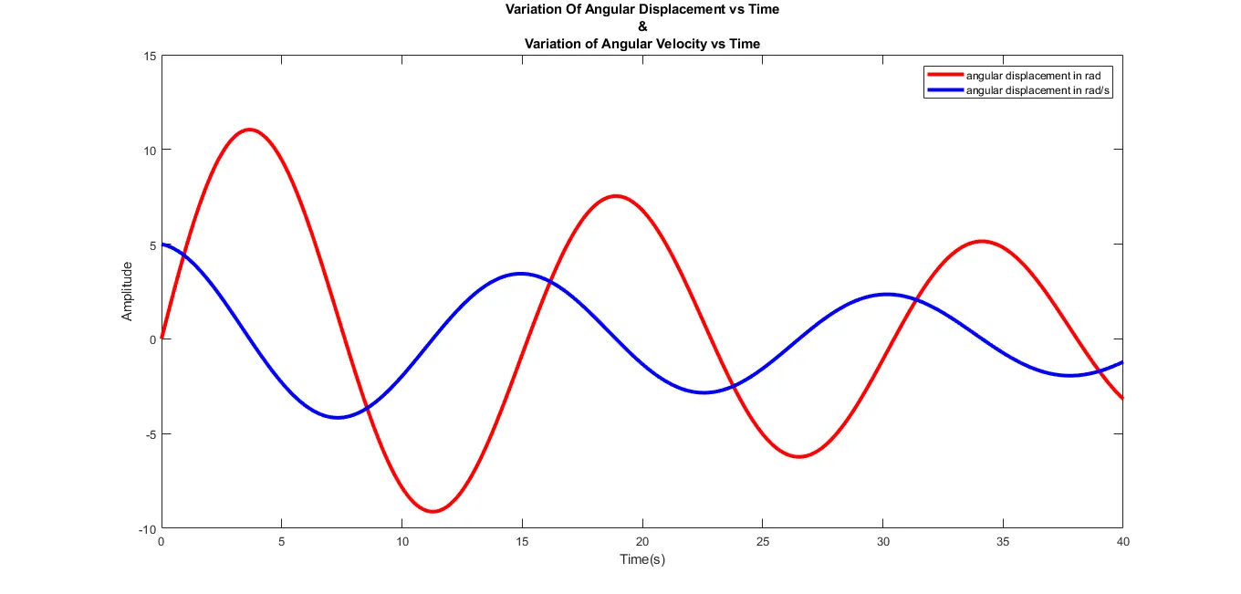
   • theta_0 specifies the initial conditions for the pendulum, with an initial angular displacement of 0 radians (theta_0(1) = 0) and an initial angular velocity of 5 rad/s (theta_0(2) = 5).

3. Time Points:

   • t_span defines a time vector using linspace, ranging from 0 to 20 seconds with 550 time points.

4. Solving the Ordinary Differential Equation (ODE):

   • The ode45 solver is used to numerically solve the ODE for the given initial conditions and time span. The ODE is defined by the function ode_func, which you should have defined elsewhere in your code. This function represents the equation of motion for the damped pendulum.

5. Plotting:

   • The code creates a plot of time versus angular displacement (results(:,1)) and angular velocity (results(:,2)) using plot.
   • Labels, a title, and a legend are added to the plot to make it informative.

6. Initialization for Animation:

   • A second figure (figure(2)) is created for the animation.
   • The loop variable ct is initialized to 1 for indexing the animation frames.

7. Animation Loop:

   • A for loop iterates over the time points stored in results.
   • For each time step, it calculates the x and y positions of the pendulum bob based on the angular displacement.
   • It then plots the pendulum's support rod, pendulum length, fixed point, and pendulum bob's position.
   • The animation frame is captured using getframe, and the frame is stored in the M array.
   • A pause of 0.002 seconds is added to control the animation speed.

8. Playing the Animation:

   • After capturing all frames, the code plays the animation using the movie function.

9. Saving the Animation to a Video File:

   • It creates a VideoWriter object named videofile for saving the animation to a video file called "Pendulum.avi."
   • The video file is opened with open(videofile).
   • The animation frames stored in M are written to the video file using writeVideo.
   • Finally, the video file is closed with close(videofile).

Function code Explanation:

• function [dtheta_dt] = ode_func(t, theta, b, g, l, m) defines a function called ode_func that takes six input arguments: t, theta, b, g, l, and m. It returns the time derivatives of the angular displacement and angular velocity as a column vector dtheta_dt.
• These lines extract the values of theta(1) and theta(2) from the input vector theta. theta(1) represents the angular displacement, and theta(2) represents the angular velocity.
• This line calculates the time derivative of the angular displacement theta1. It's simply the angular velocity theta2.
• This line calculates the time derivative of the angular velocity theta2. It's determined by two terms:
  • The first term - (b/m) * theta2 represents the damping effect. It's proportional to the angular velocity theta2 and is scaled by the damping coefficient b and the mass m.
  • The second term - (g/l) * sind(theta1) represents the gravitational force acting on the pendulum. It's proportional to the sine of the angular displacement theta1, scaled by the gravitational acceleration g, and divided by the pendulum length l.
• This line assembles the calculated derivatives dtheta1_dt and dtheta2_dt into a column vector dtheta_dt. The first element of the vector is the time derivative of angular displacement, and the second element is the time derivative of angular velocity.

Main Code:

% second order derivation
clear all
close all
clc

�fine input parameters for the pendulum
b = 0.05;   �mping coefficient
g = 9.81;   �celeration due to gravity
l = 1;      % Length of the pendulum
m = 1;      % Mass of the pendulum bob

�fine the initial conditions for the pendulum:
% - Initial angular displacement (theta_0(1)) = 0 radians
% - Initial angular velocity (theta_0(2)) = 5 radians per second
theta_0 = [0; 5];

�fine time points for simulation from 0 to 20 seconds with 550 time steps
t_span = linspace(0, 20, 550);

% Solve the ordinary differential equation (ODE) that represents the pendulum motion
% The ODE is solved using ode45, and the results are stored in 't' and 'results'
[t, results] = ode45(@(t, theta) ode_func(t, theta, b, g, l, m), t_span, theta_0);

% Create a plot of time versus angular displacement and angular velocity
figure(1); % Create a new figure for the plot
plot(t, results(:, 1), 'color', 'r', 'linewidth', 3) % Angular displacement
hold on
plot(t, results(:, 2), 'color', 'b', 'linewidth', 3) % Angular velocity
xlabel('Time (s)')
ylabel('Amplitude')
title({'Variation Of Angular Displacement vs Time', '&', 'Variation of Angular Velocity vs Time'});
legend('Angular Displacement (rad)', 'Angular Velocity (rad/s)');

% Initialize the figure for animation
figure(2);

% Initialize the frame counter for the animation
ct = 1;

% Loop through the simulation results to create an animation
for i = 1:length(results(:, 1))
    x0 = 0;
    y0 = 0;
    
    �lculate the x and y positions of the pendulum bob based on the current angular displacement
    x1 = sin((results(i, 1)));
    y1 = -cos((results(i, 1)));
    
    figure(2)
    
    % Plot the supporting rod as a green line
    plot([-1 1], [0 0], 'linewidth', 3, 'color', 'g');
    
    % Set axis limits for the animation
    axis([-2 2, -2 2]);
    
    % Plot the pendulum rod as a blue line
    line([x0 x1], [y0 y1], 'linewidth', 4, 'color', 'b');
    hold on
    
    % Plot the fixed point as a yellow circle
    plot(x0, y0, 'o', 'markersize', 6, 'markerfacecolor', 'k');
    
    % Plot the pendulum bob as a red circle
    plot(x1, y1, 'o', 'markersize', 14, 'markerfacecolor', 'r');
    
    % Set titles and legends for the animation
    title('Damping of the simple pendulum')
    legend('Support Rod', 'Length of Pendulum', 'Fixed Point', 'Pendulum Bob')
    grid on
    
    % Create a title string with the current time
    titlestring = ['Pendulum motion at time t=', num2str(t(i)), ' seconds'];
    title(titlestring, 'fontsize', 10);
    
    hold off
    
    �pture the current frame
    M(ct) = getframe(gcf);
    
    % Pause briefly to control the animation speed
    pause(0.002)
    
    % Increment the frame counter
    ct = ct + 1;
end

% Play the animation using the captured frames
movie(M)

% Create a VideoWriter object for saving the animation to a video file
videofile = VideoWriter('Pendulum.avi', 'Uncompressed AVI');

% Open the video file for writing
open(videofile)

% Write the captured frames to the video file
writeVideo(videofile, M)

% Close the video file
close(videofile)

Function Code:

function [dtheta_dt] = ode_func(t,theta,b,g,l,m)

theta1 = theta(1);
theta2 = theta(2);
dtheta1_dt = theta2;
dtheta2_dt = -(b/m)*theta2 - (g/l)*sind(theta1);
dtheta_dt = [dtheta1_dt; dtheta2_dt];
end

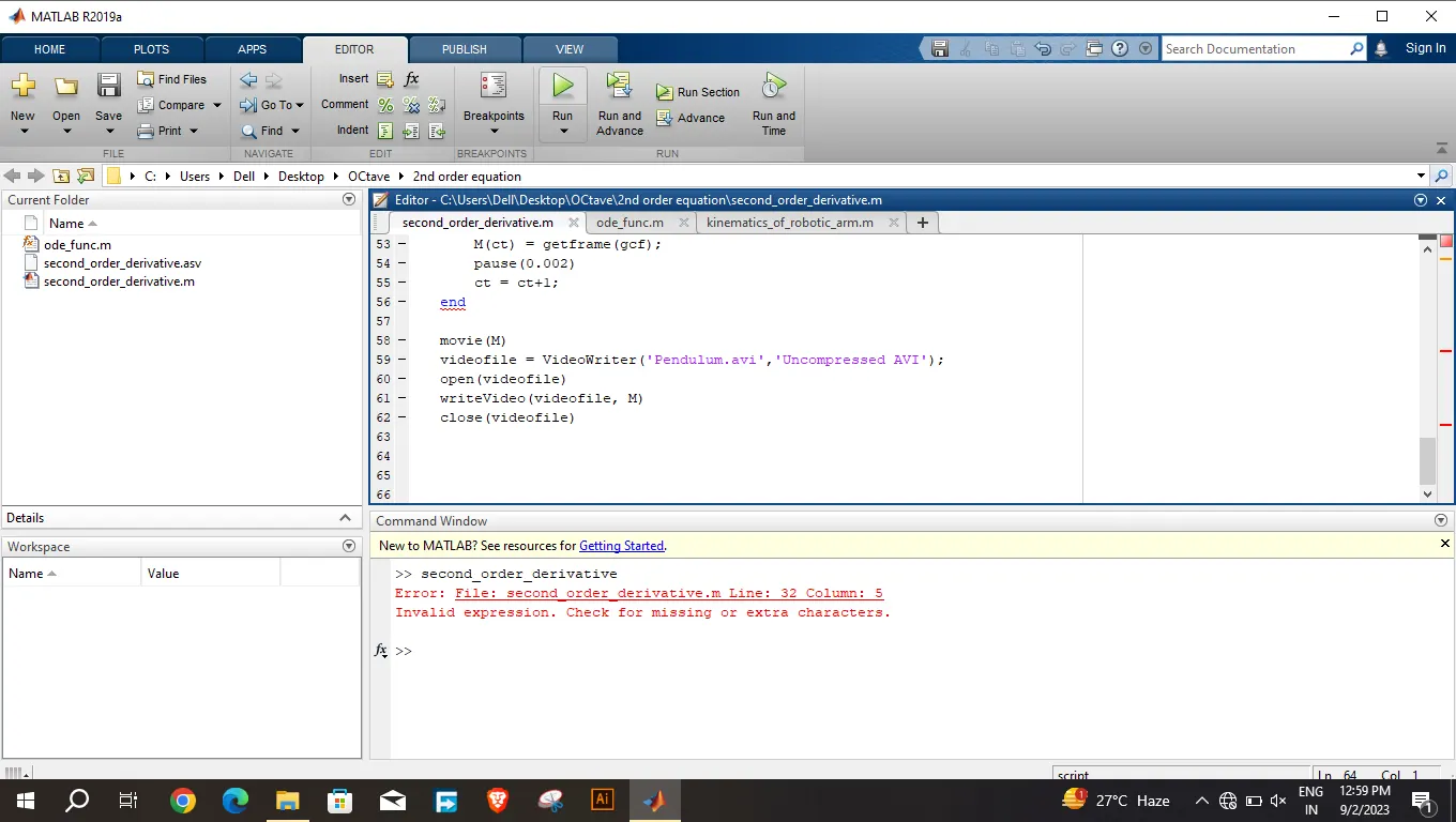
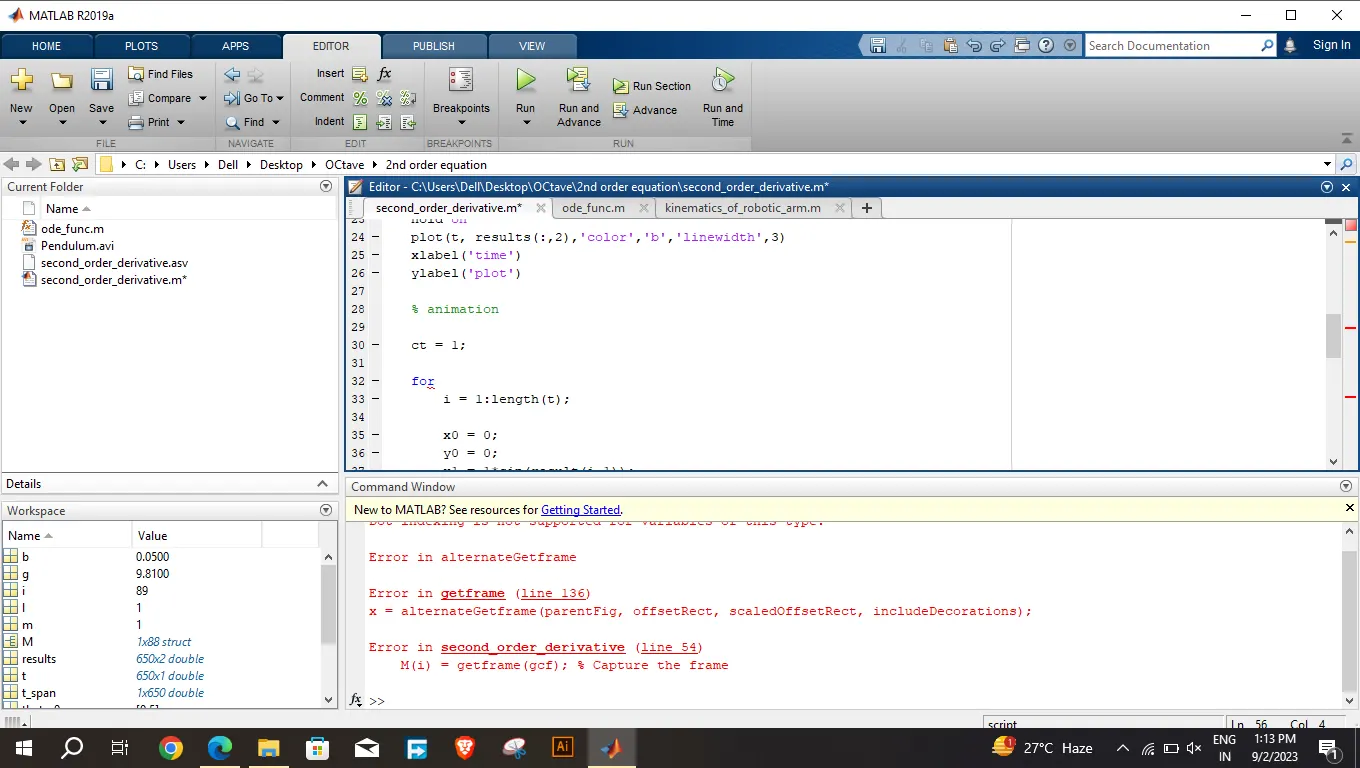
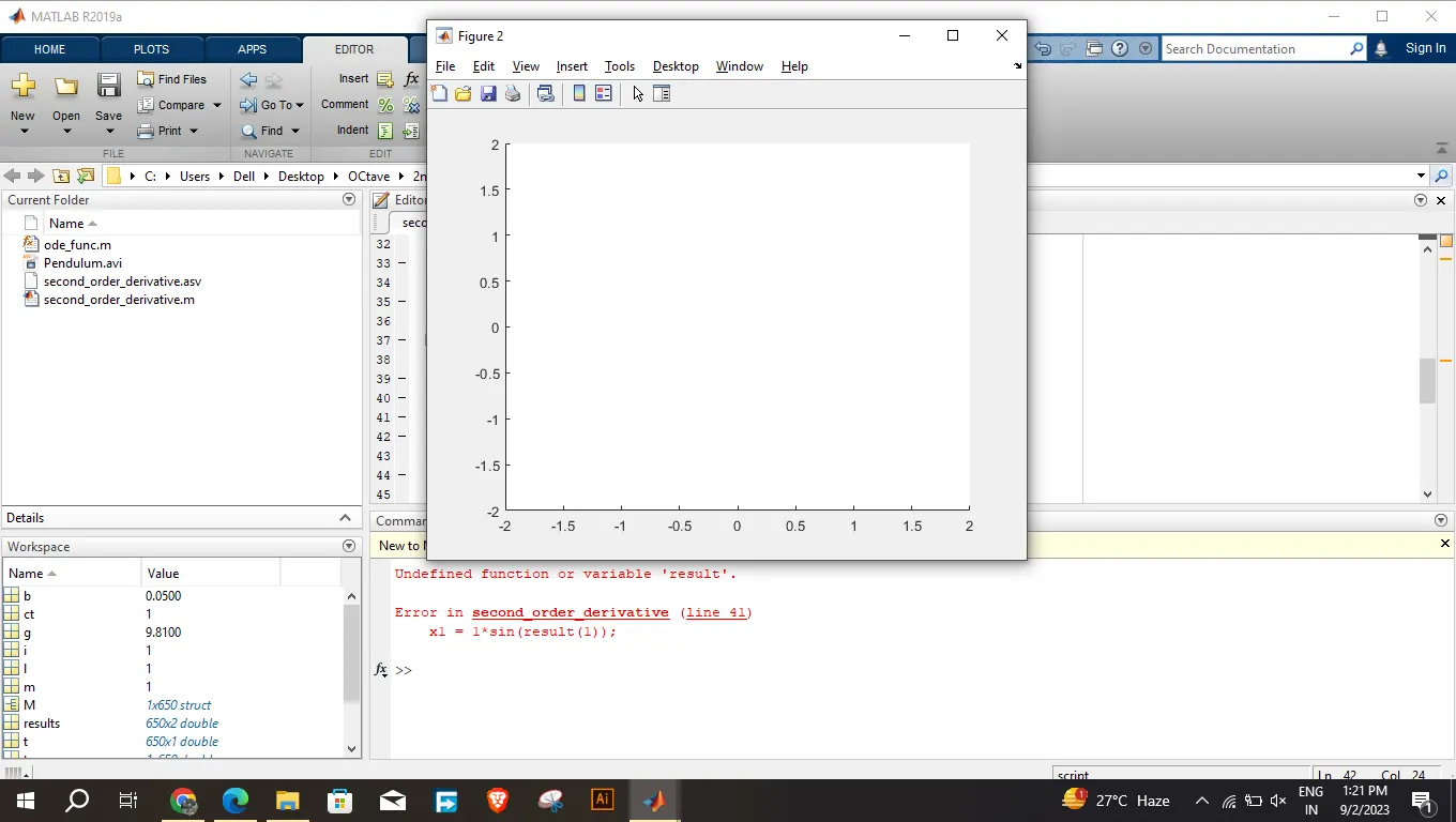
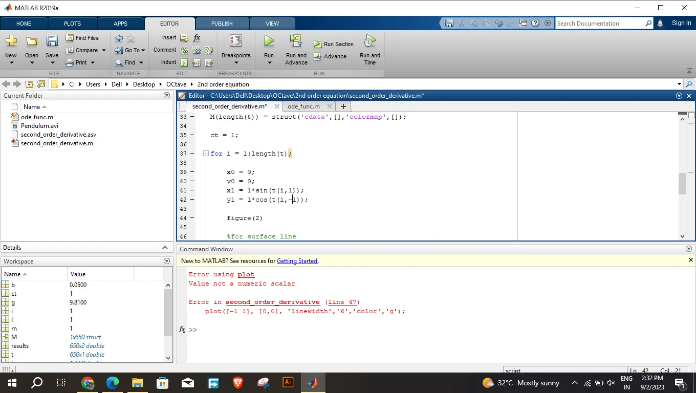
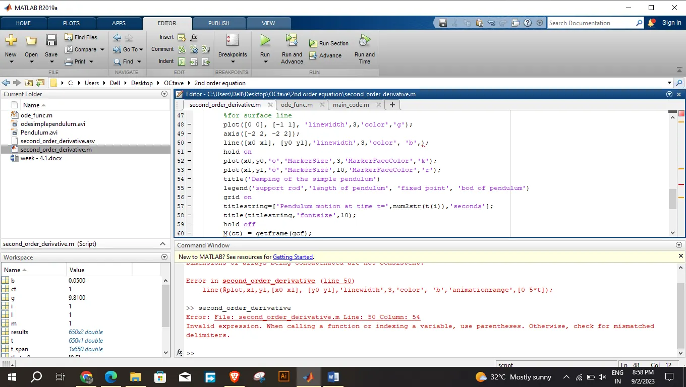
•  Errors faced while programming.

1. i = 1:length(result(:, 1))
2. x1 = sin((result(i, 1)));
y1 = -cos((result(i, 1)));
3. plot([-1 1], [0 0], 'linewidth', '3', 'color', 'g');

•  How have you overcome those errors.

1. i = 1:length(results(:, 1))
2. x1 = sin((results(i, 1)));
y1 = -cos((results(i, 1)));
3. plot([-1 1], [0 0], 'linewidth', 3, 'color', 'g');

•  Screenshots showing errors thrown in command window.

Results:

Plot:

Youtube Link:

<iframe src="https://www.youtube.com/embed/jtk__GNxlR4" allowfullscreen="allowfullscreen"></iframe>

Conclusion:

1. ODE has been solved using ode45 in MATLAB
2. Motion of simple pendulum has been animated.
3. It was observed that as damping co-efficient increses ,motion of pendulum gets damped faster
4. And from the above mentioned examples we can understand that damping has both advantages and disadvantages.