Week 4.1 - Solving second order ODEs

CODE:

clear all
close all
clc

%INPUTS

g = 9.8;      %Acceleration due to gravity, m/s^2
l = 1;        %Length of the pendulum, m
m = 1;        %Mass of the pendulum, kg
p1 = 0;       %Initial position in radians
v1 = 3;       %Initial velocity in rad/sec
t1 = 20;      %Time span for result calculation, sec
c = 0.05;     %Damping coefficient

%INITIAL CONDITIONS
theta_0=[p1;v1];

%CREATING 500 TIME POINTS IN THE GIVEN TIME PERIOD
t_span=linspace(0,t1,500);

%Solve ODE
[t,results]=ode45(@(t,theta) simplependulum_equn(g,l,c,theta,t),t_span,theta_0);

%Configure the video writer
VideoFile = VideoWriter('simple_pendulum_anil.avi','Uncompressed AVI');
open(VideoFile)

%Start plotting the results to create a video
for k = 1:500
    
    x1=0;
    y1=0;
    x2=l*sin(results(k,1));
    y2=-l*cos(results(k,1));
    x=-2*l;
    y=2*l;
    z=-2*l;
    plot([0,0],[z,0],'--',[x1,x2],[y1,y2],x2,y2,'go','color','k',...
    'linewidth',2,'markersize',20,'markerfacecolor','g','markeredgecolor','g');
    axis([x y z 0]);
    daspect([1 1 1]);%To ensure same scales along both the axes.
    xlabel('Length in meter');
    ylabel('Length in meter');
    title([num2str(t_span(k)),'s'])
    pause_t=t1/500;
    pause(pause_t);
    M = getframe(gcf);
    writeVideo(VideoFile,M)
    
end

close(VideoFile)

%THE FOLLOWING FUNCTION PROVIDES THE SYSTEM OF FIRST ORDER DIFFERENTIAL EQUATIONS TO
%THE ODE45 SOLVER
function [dtheta_dt]= simplependulum_equn(g,l,c,theta,t)

    w=g/l;
    theta1=theta(1);
    theta2=theta(2);
    dtheta1_dt=theta2;
    dtheta2_dt=-w*sin(theta1)-(c/l)*theta2;
    dtheta_dt=[dtheta1_dt;dtheta2_dt];

end

EXPLANATION:

First, all the input variables are assigned respective values as specified in the problem.

The function simplependulum_equn available at the end of the code takes the input variables along with dependent variables (theta_1 and theta_2) and returns the ODE in the form of a system of first-order differential equations.

Finally, the respective arguments (function handle to simplependulum_equn function , time span and initial condition vector) are passed to the ode45 solver to finally obtain the solution of the differential equation in t and results matrices

The solver returns angle (theta_1) and angular velocity(theta_2) as the output in the results vector at each time point corresponding to the value stored in the t vector.

1. clear all, close all, clc: These commands clear the workspace, close all open figures, and clear the command window.

2. Input Parameters: The code sets up various parameters for the simple pendulum motion:

   • g: Acceleration due to gravity (m/s^2).
   • l: Length of the pendulum (m).
   • m: Mass of the pendulum (kg).
   • p1: Initial position of the pendulum in radians.
   • v1: Initial velocity of the pendulum in rad/sec.
   • t1: Time span for result calculation in seconds.
   • c: Damping coefficient (a value to simulate damping effects).

3. Initial Conditions: The initial position and velocity of the pendulum are stored in the theta_0 variable.

4. Time Span: The time span for which the simulation will be run is defined using linspace to create 500 equally spaced time points between 0 and t1. This will be used as the input to the ODE solver.

5. Solving Ordinary Differential Equation (ODE): The code uses the ode45 solver to numerically solve the simple pendulum's differential equations. The function simplependulum_equn provides the system of first-order differential equations needed for the ODE solver.

6. Video Configuration: The code sets up a video writer named VideoFile for creating a video of the pendulum's motion.

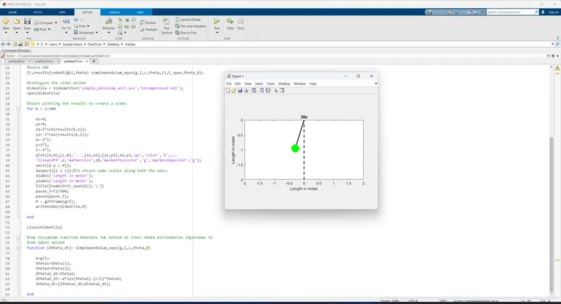
7. Animation Loop: The for loop runs 500 times, corresponding to the 500 time points. In each iteration, the position of the pendulum is updated, and the pendulum's configuration is plotted. The plot includes a dashed vertical line representing the pivot point, a solid line representing the pendulum rod, and a green circle at the pendulum's bob.

8. Video Recording: In each iteration, the plot is captured as a frame using the getframe function, and the frame is written to the video file using the writeVideo function.

9. Closing the Video File: After the animation loop finishes, the video file is closed using the close function.

10. The function simplependulum_equn: This function defines the system of first-order differential equations that describe the simple pendulum's motion. It takes g, l, c, theta, and t as input arguments and returns the first derivatives of theta with respect to time, dtheta_dt.

The screenshot of the execution is attached below

SCREENSHOT:

YOU TUBE LINK : https://youtu.be/oMH-zYN42PY