Week 4.1 - Solving second order ODEs

In Engineering, ODE is used to describe the transient behavior of a system. A simple example is a pendulum

The way the pendulum moves depends on the Newtons second law. When this law is written down, we get a second order Ordinary Differential Equation that describes the position of the "ball" w.r.t time.

Similarly, there are hundreds of ODEs that describe key phenomena and if you have the ability to solve these equations then you will be able to simulate any of theses systems.

Your objective is to write a program that solves the following ODE. This ODE represents the equation of motion of a simple pendulum with damping

In the above equation,

g = gravity in m/s2,

L = length of the pendulum in m,

m = mass of the ball in kg,

b=damping coefficient.

Write a program in Matlab\Octave that will simulate the pendulum motion, just like the one shown in the start of this challenge.

use,

L=1 metre,

m=1 kg,

b=0.05.

g=9.81 m/s2.

Simulate the motion between 0-20 sec, for angular displacement=0,angular velocity=3 rad/sec at time t=0.

When you do this you will get the position of the pendulum as a function of time. Use this information to animate the motion of the pendulum, as shown in the below figure.

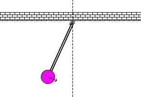
Your animation does not have to look exactly like this and here is the logic.

• For each value in time
• Create an image that represents the position of the pendulum
• You can assume the length of the string and the size of the ball
• Use the marker command to create a sphere
• One end of the pendulum is fixed
• The other end moves according to the solution of the ODE you had solved.
• If you are using using Matlab, use the movie command create an animation
• If you are using Octave you need to generate images first and then stitch them to form the animation (https://skilllync1.freshdesk.com/support/solutions/articles/43000012529-creating-animations-in-octave)

• Upload an animation on You tube and provide the You tube link for an animation in your report.

2. Submit a report that has the following content:

• Step wise explanation of your code.
• Errors faced while programming.
• How have you overcome those errors.
• Screenshots showing errors thrown in command window.

The presentation of your code will be taken into consideration while grading. Labelling sections of your code using comments is appreciated.

Upload the code using "INSERT SAMPLE CODE" option and then post screenshot of the plots generated.

In case if you are not able to finish the challenge, upload until what you have done and explain the procedure and plot. Deserved marks will be allotted.

GENERAL INSTRUCTIONS:

• The codes, plots, images, GIFs, and videos should be submitted only through the answer box.
• Use the Google Drive to share only the cad models or other answers which couldn't be done through the answer box.

NOTE:

• Violating the above instructions will lead to ZERO marks.
• Link sharing should be enabled while sharing the Google Drive link, else the challenge will be awarded ZERO marks.

Just submitting your code without the report will result in a 0 grade

AIM:- To show a animation of damped simple pendulum oscillations animation

EXPLAINATION:-

first we solve the 2nd order differential equation of a damped simple pendulum.

%function
function [dtheta_dt] = ode_fun2(t, theta, b,g,l,k)
theta1 = theta(1);
theta2 = theta(2);
dtheta1_dt = theta2;
dtheta2_dt = -(b/k)*theta2-(g/l)*sin(theta1);
dtheta_dt = [dtheta1_dt; dtheta2_dt];
end

%main script
% 2ODE
b = 0.05;
g =9.81;
l = 1;
k = 1;

%initial_condition i.e solution matrix (ang dis. = 0, ang vel.=5)
theta_0 = [0; 3];

%time_points

t_span = linspace(0,10,500);

%solve ODE

[t, results] = ode45(@(t,theta) ode_fun2(t, theta, b,g,l,k),t_span, theta_0);
%results = [angular displacement, angular velocity]
plot(t,results(:,1))
hold on
plot(t,results(:,2))
xlabel('plot')
ylabel('time')
%%Animation
x0 = 0;
y0 = 0;

ct = 1; % frame for every second

for i = 1:length(t)
     x1 = l*sin(results(i,1));
     y1 = -l*cos(results(i,1));
     figure(2)
     plot([-1 1],[0 0],'linewidth',6,'color','g');
     axis([-2 2 -2 2]);
     line([x0 x1],[y0 y1],'linewidth',2,'color','b');
     hold on;
     plot(x0,y0,'o','markersize',3,'markerfacecolor','y');
     plot(x1,y1,'o','markersize',5,'markerfacecolor','r');
     title('damped simple pendulum');
     legend('support rod','length of pendulum','fixed point','bob of pendulum');
     grid on;
     hold off;
     M(ct)=getframe(gcf);
     ct=ct+1;
end
%creating a movie for pendulum oscillations
movie(M);
videofile=videowriter('pendulum_avi','uncompressed AVI');
open(videofile);
writeVideo(videofile,M);
close(videofile);