Week 4.1 - Solving second order ODEs

A.I.M:

To write a program that solves the following ODE. This ODE represents the equation of motion of a simple pendulum with damping

In the above equation,

g = gravity in m/s2,

L = length of the pendulum in m,

m = mass of the ball in kg,

b=damping coefficient.

Write a program in Matlab\Octave that will simulate the pendulum motion, just like the one shown at the start of this challenge.

use,

L=1 metre,

m=1 kg,

b=0.05.

g=9.81 m/s2.

Simulate the motion between 0-20 sec, for angular displacement=0,angular velocity=3 rad/sec at time t=0.

SOLUTION:

MATLAB CODE FOR PENDULUM SIMULATION:

% Matlab code to simulate pendulum motion.
% 2nd order ordinary differential equation used:
% d^2.theta/d.t^2 + b.d.theta/m.d.theta + g.sin.theta/L = 0

close all % It is used to close the all current plots.
clear all % It is used to clear the workspace.
clc % It is used to clear the commond window.

% Inputs of a Problem to be solved
l = 1;      % Length of the pendulum in (m),
m = 1;      % Mass of the ball in (kg),
b = 0.05;   % Damping coefficient,
g = 9.81;   % Gravity in (m/s).

% Initial conditions
theta_0 = [0;3];

% Time points
t_span = linspace(0,20,300); % linespace command is used to give time span from 0 to 20 by the interval of 300

% Solve ODE using ode45
[t, results] = ode45(@(t,theta) ode_func(t, theta, b, g, l, m), t_span, theta_0);
%Using  ode45 command, we can create a anonymus function of variable
%(t,theta) and solving the ode_func whose inputs are (t, theta, b, g, l, m)
% and storing in the solutions  in matrix [t, results]. Here results is
% a matrix of multiple rows and two columns stroring the values of angular
% displacement in first column and angular velocity in second column with
% varying time. The time varied is stored in t which is a single column
% matrix.

% Plotting Angular displacement and Angulur velocity.
figure(1)
hold on % The two curves are plotted on the same figure using hold on command.
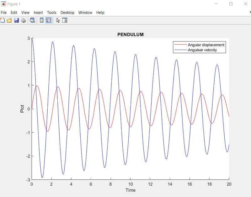
plot(t, results(:,1), 'color', 'r') % Plot for Angular displacement
plot(t, results(:,2), 'color', 'b') % Plot for Angular velocity.
xlabel('Time') % For x-axis given a time
ylabel('Plot') % For y-axis given a plot
legend('Angular displacement', 'Angulaar velocity') % It is used to distinguish the two curves inside the plot
title ('PENDULUM')

ct = 1; 

% For loop is used to plot the motion of pendulum in a single frame
for i = 1 : length(t)
    
    % Coordinates of pendulum with respect to angular displacement
    % (x0 & y0) are the giving the coordinates for the two end points of a
    % string and (x1 & y1) for each iteration of for loop. 
    x0 = 0;
    y0 = 0;
    x1 = l*sin(results(i,1));
    y1 = -l*cos(results(i,1));
    
    % Potting the pendulum movement.
    figure(2)
    plot ([x0,x1], [y0,y1]) % Plotting line between coordinates (x0,y0) & (x1,y1).
    hold on % Hold on command is used to not erase the previous plots.
    plot ([-1.5 1.5], [0 0], 'linewidth', 10, 'color', 'g') % Plotting the line between (-1.5,0) & (1.5,0)
    axis ([-1.5 1.5 -1.5 0.5]) % Fixing the plot axis between x-coordinates (-1.5,0) and y-coordinate (1.5,0.5)
    plot (x1, y1, 'o', 'markersize', 25, 'markerfacecolor', 'r') % For creating a circle of 25 size at coordinates (x1,y1) for each iteration of for loop
    pause (0.0001) % Pause of loop
    hold off % Putting off the hold on command
    
    % Capturing the frames
    M(ct) = getframe(gcf); % Creating an Array (M) and store all the frames of the plot in the array.
    ct = ct + 1; % Increment of the variable (ct) by value 1 for each iteration
end % End of for loop

% Creating a video file
movie(M); % creating a movie of array M
videofile = VideoWriter('Pendulum_simulation.avi', 'Uncompressed AVI'); % creating a video file using VideoWriter command
open(videofile); % Opening the videofile.
writeVideo(videofile, M); % To create a video of all the frames in the array M.
close(videofile); % Close the videofile.

MATLAB FUNCTION CODE FOR PENDULUM:

% Fuction code for pendulum

function [dtheta_dt] = ode_func(t, theta, b, g, l, m)

theta1= theta(1); % Storing values of angulur displacement
theta2 = theta(2); % Storing values of angular velocity

% Splitting 2nd order ODE
dtheta1_dt = theta2;
dtheta2_dt = -(b/m)*theta2 - (g/l)*sin(theta1);

% Storing the values in variable
dtheta_dt = [dtheta1_dt; dtheta2_dt];
end % commond close the function

OUTPUT FIGURE OF PENDULUM:

PENDULUM YOUTUBE VIDEO LINK:

https://youtu.be/JGZObFY5iIg