Week 4.1: Project - Steady state simulation of flow over a throttle body
AIM: To run the simulation of a steady-state simulation of flow over a throttle body.
THEORY:
A throttle body is essentially a large air valve that sits between the intake manifold and the air intake pipe. An engine has one throttle body, which bolts to the intake manifold's plenum (the large air cavity in the center). A throttle body controls airflow into the engine, a crucial factor for controlling the engine's air/fuel ratio. Throttle bodies come in several shapes, sizes, and configurations and can perform several tasks outside of their normal air-metering duties.
Throttle bodies usually use butterfly valves. These valves consist of a casing with a large hole in the center, which is
filled with a steel plate called a butterfly, or throttle plate. The throttle shaft is a rod that passes through the housing and is connected to the throttle cable on the outside and the throttle plate on the inside. When the throttle shaft turns, it rotates the throttle plate, allowing air to go around it and into the engine.
Steady-state Simulation:
A steady-state simulation is used to investigate the steady-state behavior of a system, where the simulation continues until the system reaches a steady state.
Like a steady-state model, dynamic models are based on first principles that cannot be violated. Conservation laws, phase equilibria, heat and mass transfer, and kinetics are also applied in dynamic models. The most significant difference between steady-state and dynamic simulation is that steady-state assumes that variables are constant with respect to time. This means that in a steady-state there is no accumulation in the system, so the overall mass and energy input matches its output. Conversely, dynamic models consider the mass and energy rate of accumulation within the system, which allows one to determine how long it would take to reach a stable condition starting from a specified initial state.
SETUP AND SOLUTION:
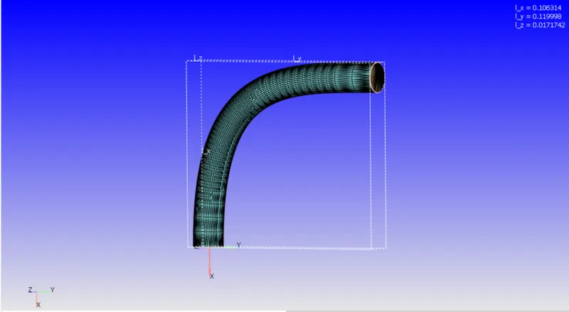
Geometry
Setup:
Application Type
Time-based
MATERIALS:
1. Gas simulation -Standard
2. Global Transport Parameters -Standard
3. Reaction Mechanism -Standard
SOLUTION PARAMETERS
Steady-state solver>Full hydrodynamic>Compressible
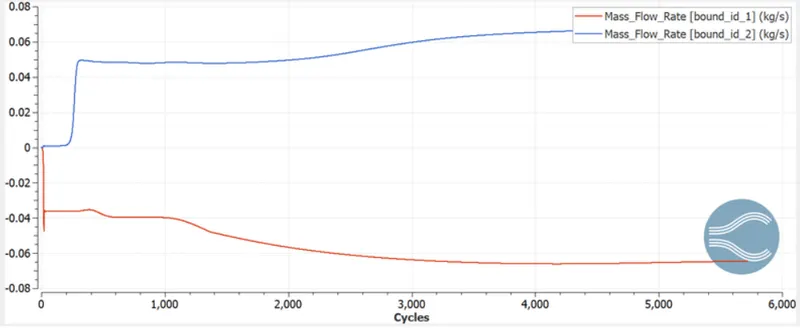
Mass flow rate
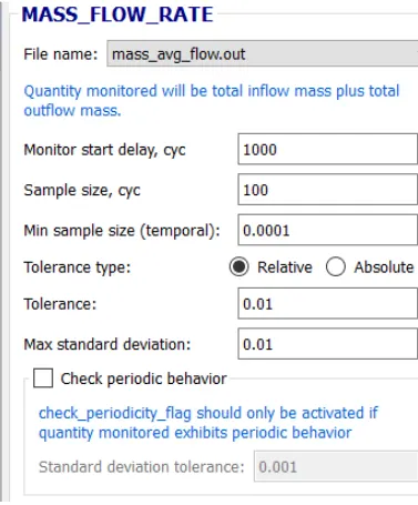
1 Run parameter
steady state monitor
2 simulation time parameter
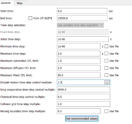
3. Solver parameters
Navis-stokes solver scheme: PISO
Navis-stokes solver type: pressure-based
Max convection CFL limit: 1
Boundary condition
1.inlet
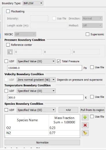
2.outlet
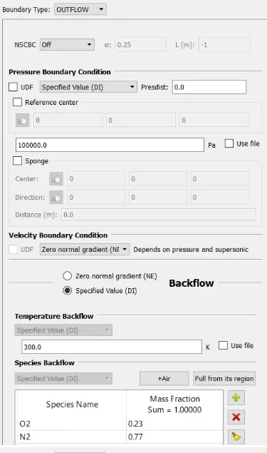
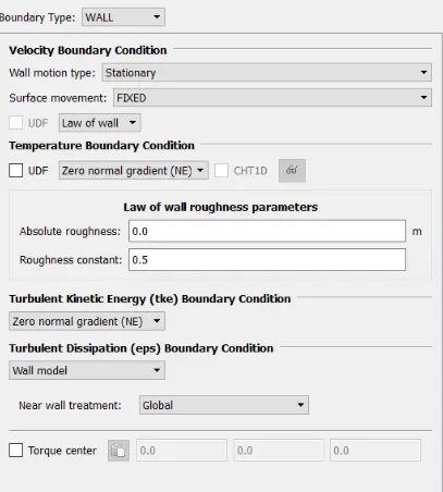
3.Elbow-wall
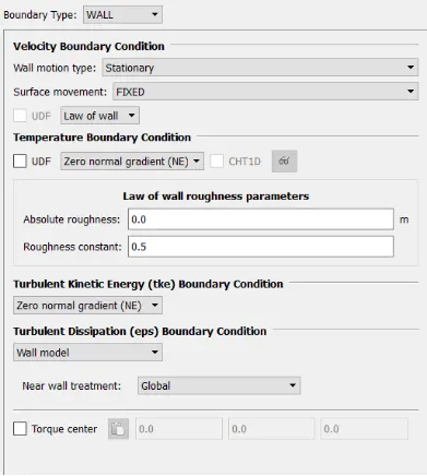
4.throttle
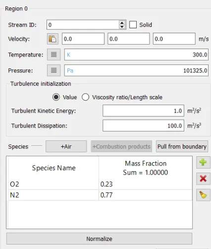
Initial conditions and events
1. Regions and initialisation
Physical model RNG k-epsilon
Grid control
1. Base mesh
dx=2e-3m dy=2e-3m dz=2e-3m
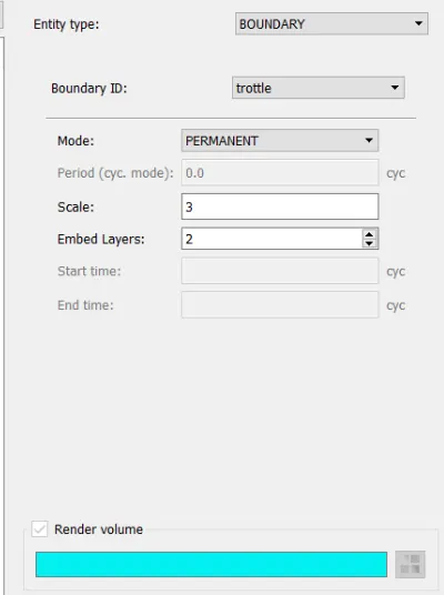
2. Fixed embeding
Output/Post processing
1. Post variable selection
standard
2. Output files
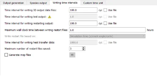
Then Export the Files
Then continuing the setup in Cygwin:
- leading to the folder where the exported files are saved
- Then using mpiexec.exe -n 2 converge.exe restricted to simulate the setup
- After the output is generated, we lead the Cygwin to the output folder, and by copying the post_convert folder and
- Using mpiexec.exe -n 2 post_convert.exe and converting these files for processable output in ParaView.
Mesh:
Solution:
Mass flow rate plot:
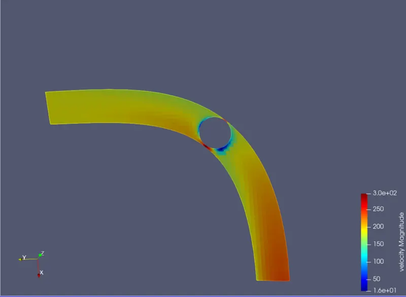
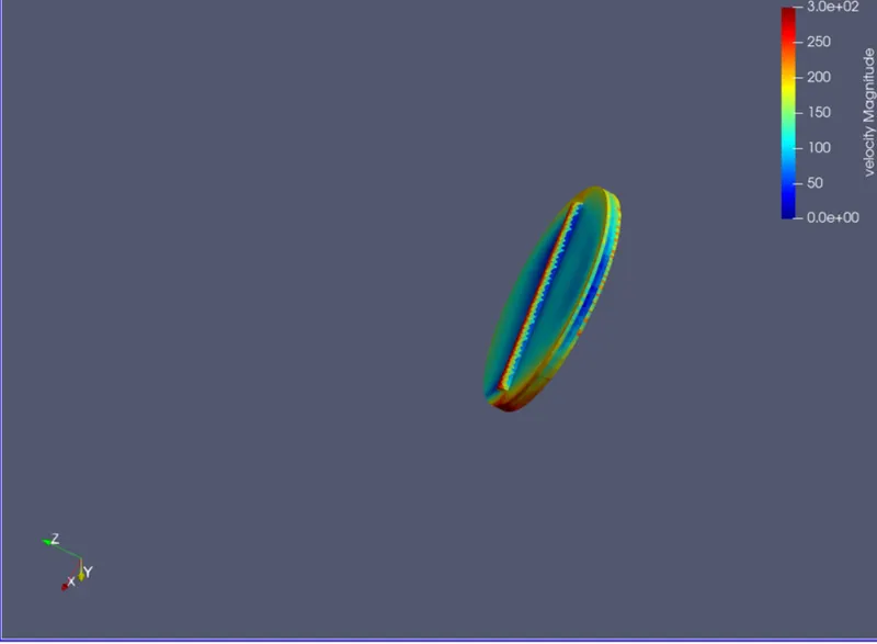
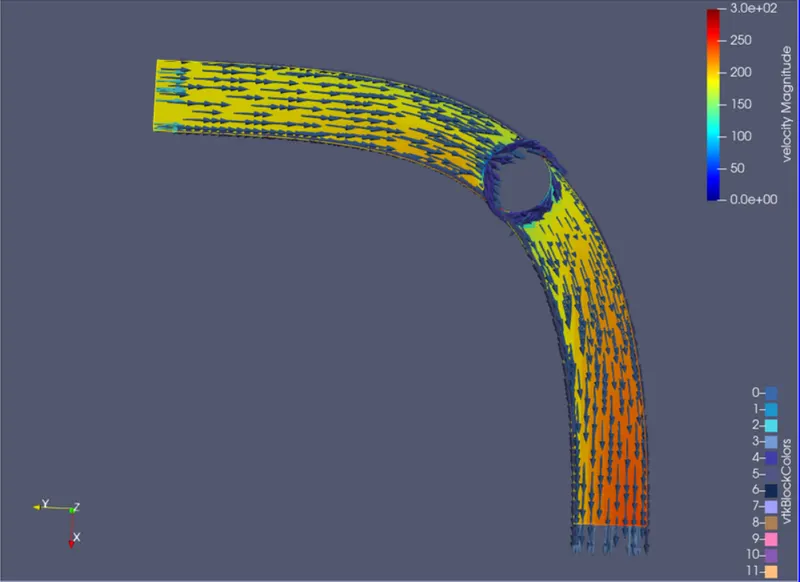
velocity contour
CONCLUSION:
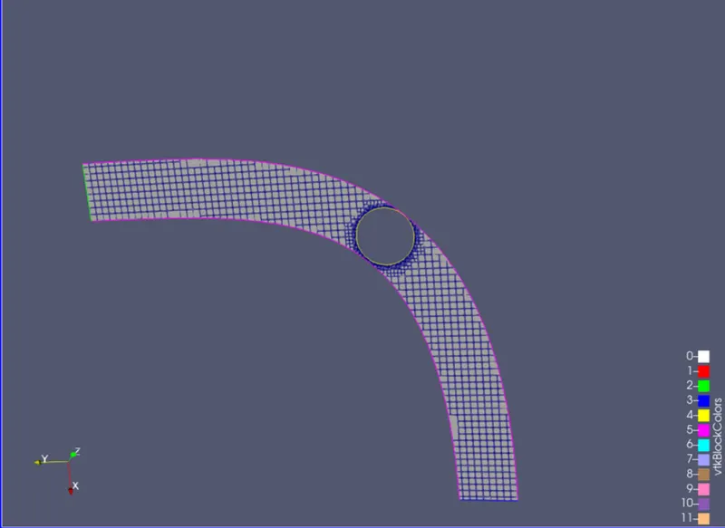
• Due to the fixed embedding of the throttle valve, the simulations near to it become clear as the number of cell count got increased in the specified region.
• The velocity increases near the elbow valve since the area is less and pressure gets dropped in the region which causes the velocity to increase.
• The velocity of the fluid decreases when it collides with the throttle valve.
• It also causes the formation of the stagnation point due to an increase in the pressure and decrease of velocity.