Week 4.1: Project - Steady state simulation of flow over a throttle body
Aim:
To Set up and run the steady state simulation for flow over throttle body.
Objective:
Post process the results and show pressure and velocity contours.
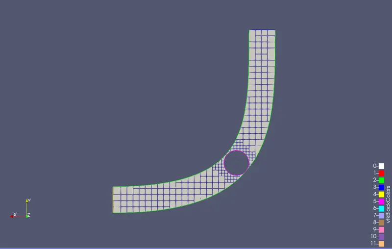
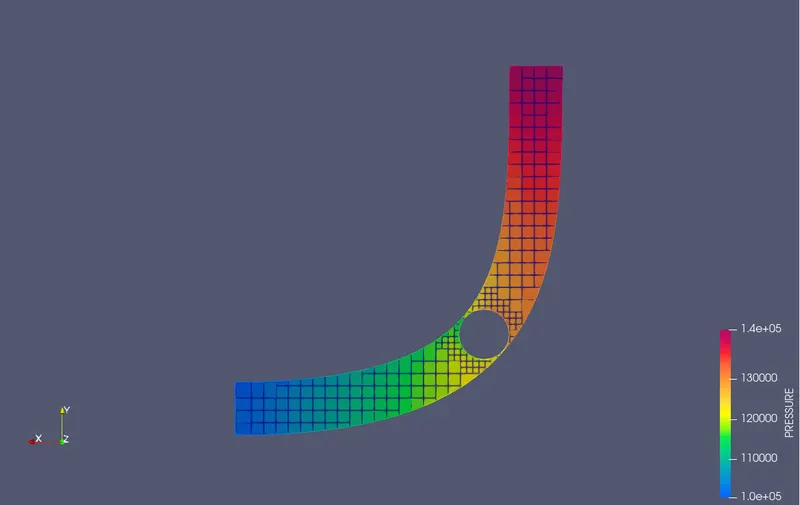
Show the mesh (i.e surface with edges)
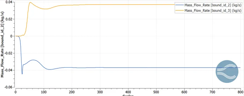
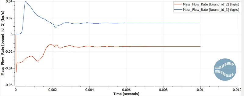
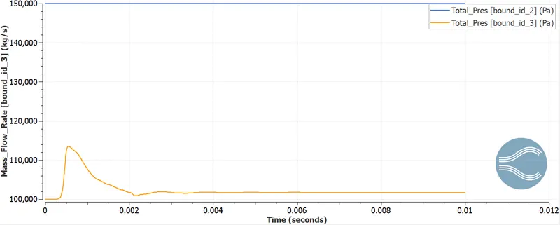
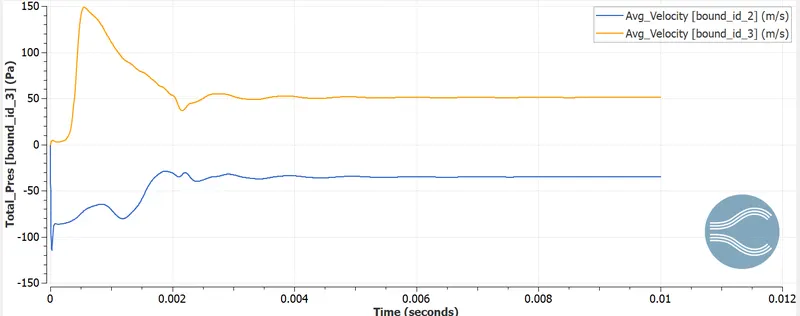
Show the plots for pressure, velocity, mass flow rate and total cell count.
Create an animation in which it throttle movement should be visible.
Theory:
Introduction:
A throttle body is actually an oversized air valve that sits between the manifold and also the air intake pipe. Associate in Nursing engine has one throttle body, that bolts to the intake manifold\'s plenum (the giant air cavity within the center). A throttle body controls flow into the engine, a vital issue for dominant the engine\'s air/fuel quantitative relation. Throttle bodies are available many shapes, sizes, and configurations and may perform many tasks outside of their traditional air-metering duties.
Throttle bodies sometimes use butterfly valves. These valves incorporates a casing with an oversized hole within the center, that is full of a plate referred to as a butterfly, or throttle plate. The throttle shaft may be a rod that passes through the housing and is connected to the throttle cable on the skin and also the throttle plate on the within. once the throttle shaft turns, it rotates the throttle plate, permitting air to travel around it and into the engine.
Steady state flow:
A steady-state simulation is employed to analyze the steady-state behavior of a system, wherever the simulation continues till the system reaches a steady-state.
Like a steady-state model, dynamic models area unit supported 1st principles that can't be profaned. Conservation laws, part equilibria, heat and mass transfer, and dynamics also are applied in dynamic models. the foremost important distinction between steady-state and dynamic simulation is that steady-state assumes that variables area unit constant with relation to the time. this suggests that in steady-state there's no accumulation within the system, that the overall mass and energy input matches its output. Conversely, dynamic models think about the mass and energy rate of accumulation among the system, that permits one to work out however long it might fancy reach a stable condition ranging from a given initial state. Figure 2, below, represents the simulation scope for steady-state and dynamic simulation models.
Case setup: Preprocessing
Case Set-up: General Flow
Materials:
Predefined Mixtures: Air
(Gas Simulation)
Simulation Parameters
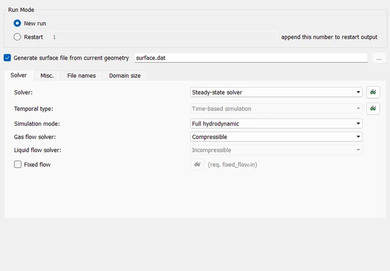
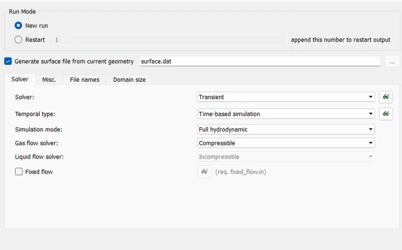
Solver: Pressure-based steady problem solver
Mode: Full Hydronic
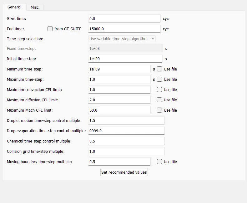
Start time: zero cycles
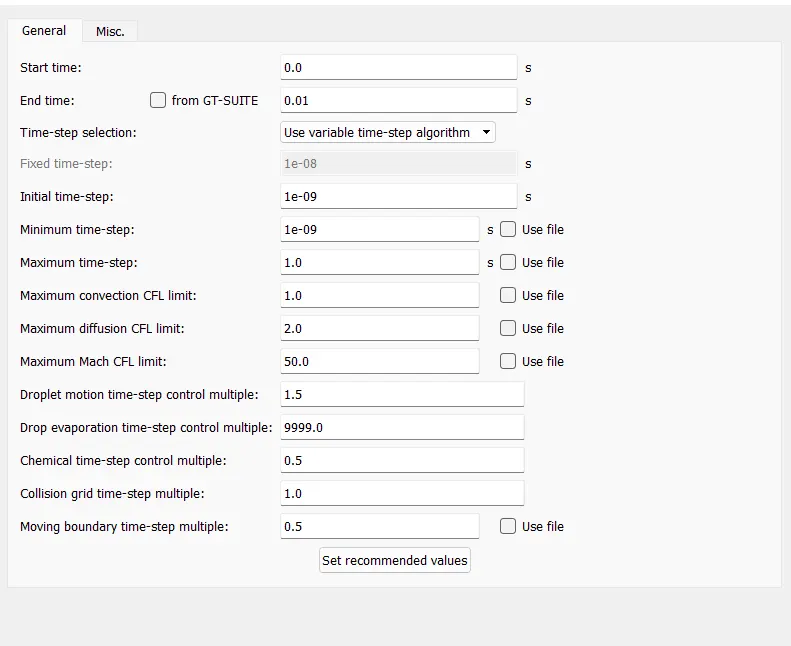
End time: 15000 cycles
Initial time-step: 1e-9 s
Minimum time step: 1e-9 s
Maximum time step: one.0 s
Regions and initialisation
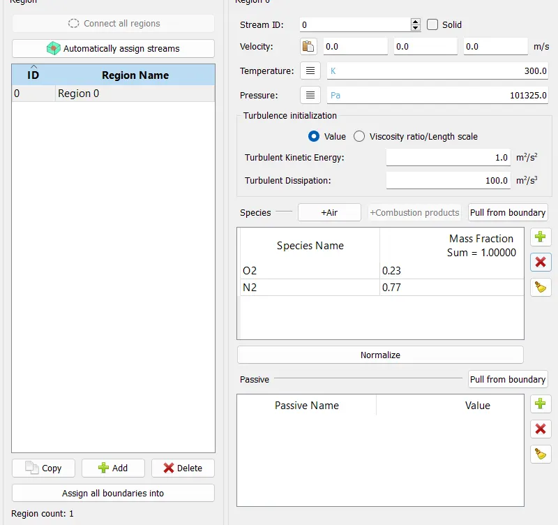
Added Region (Air)
Pressure: 101325 Pa
Species: Air - O2 = zero.23, N2 = 0.77
Boundary Conditions
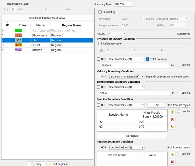
Inlet: influx 150000 Pa Air
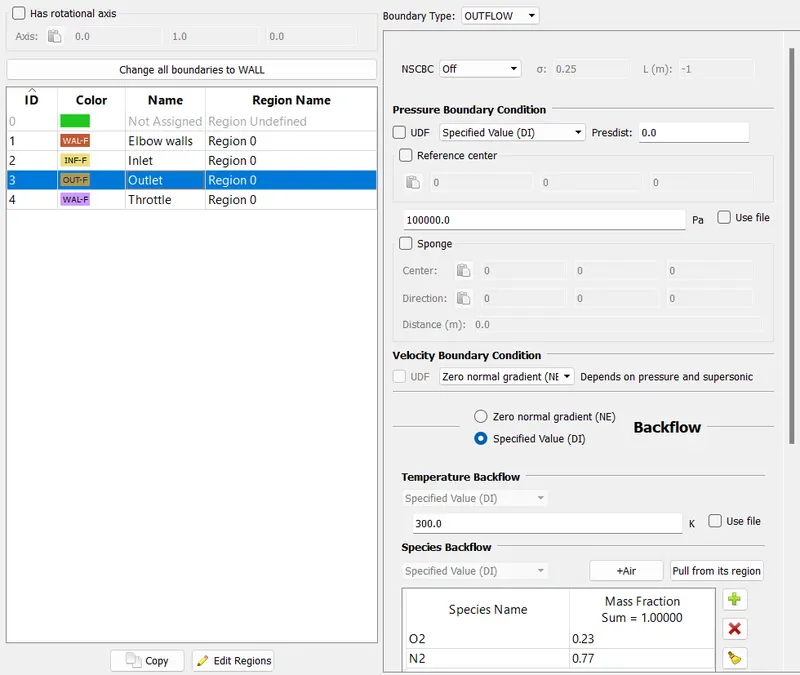
Outlet: Outflow 101325 Pa Air
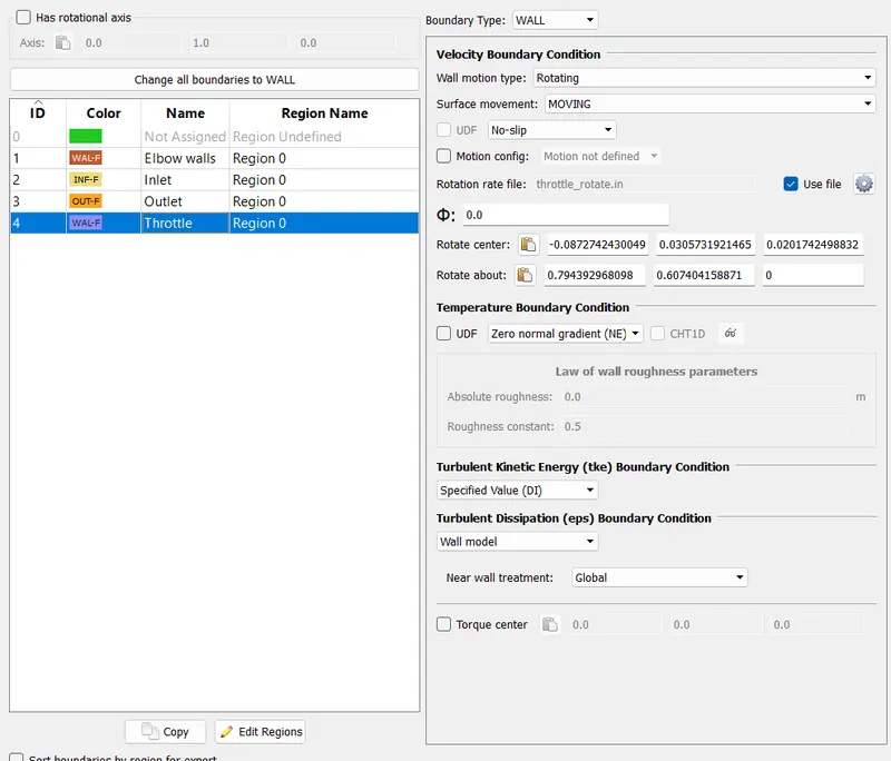
Throttle and Elbow wall: Wall
Velocity boundary conditions: Law of wall
Wall motion type: Stationary
Surface Movement: mounted
Temperature boundary conditions: Law of wall (300K)
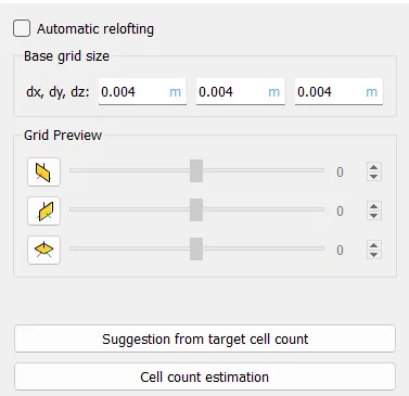
Base Grid: Mesh in dx, metallic element and dz directions = zero.002
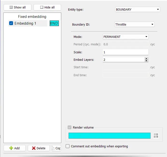
Fixed Embedding
Fixed embedding is employed to refine the mesh round the desired regions. during this case, the regions of interest area unit the inner walls of the channel. Therefore, the mounted embedding is applied with a scale of three and a couple of embedded layers.
Output files:
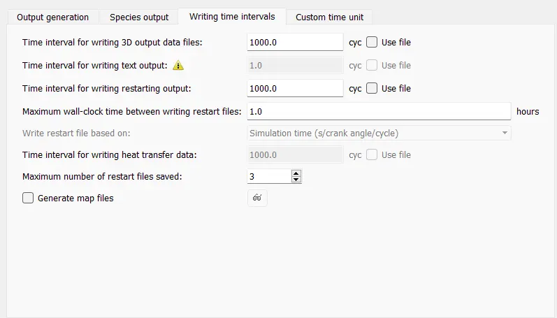
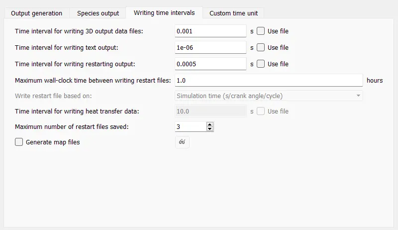
Time interval to put in writing 3D output knowledge files- one thousand.0 cycles
This means that when each one thousand cycles, 3D output knowledge files are written and saved. Since we tend to area unit running the simulation for 15000 cycles, we tend to shall have fifteen 3D output knowledge files.
Converge model:
Result: Paraview
RESULT:
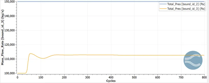
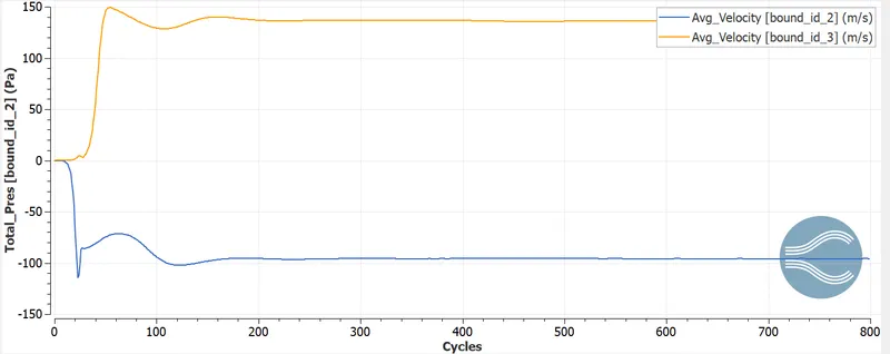
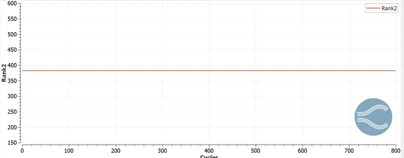
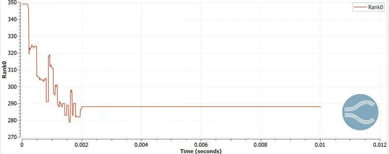
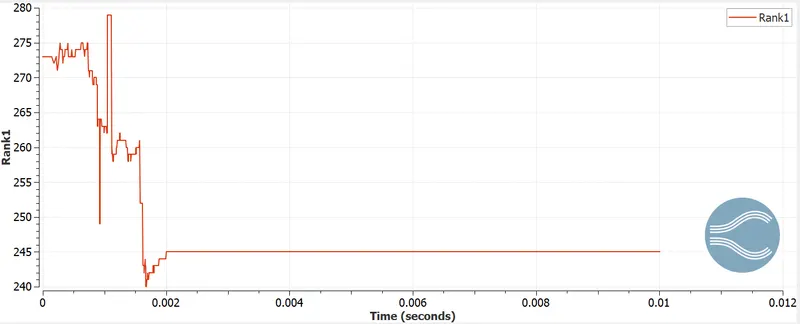
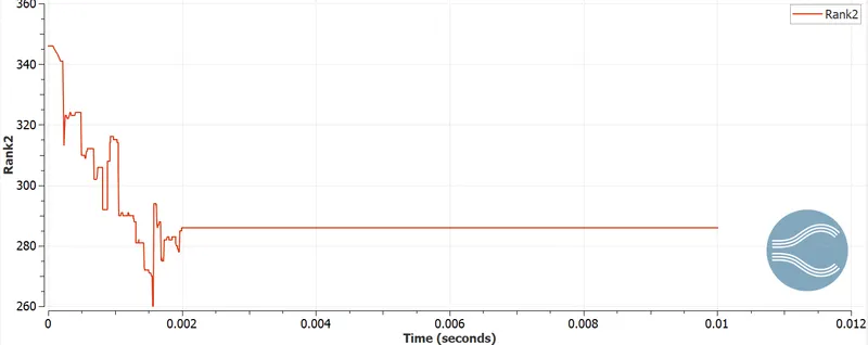
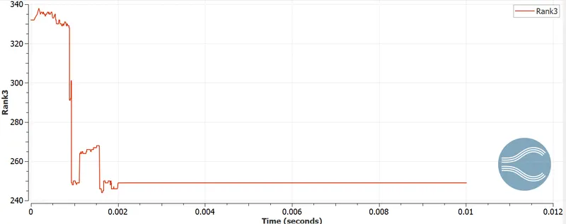
Rank cycles:
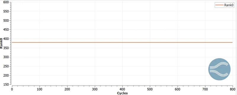
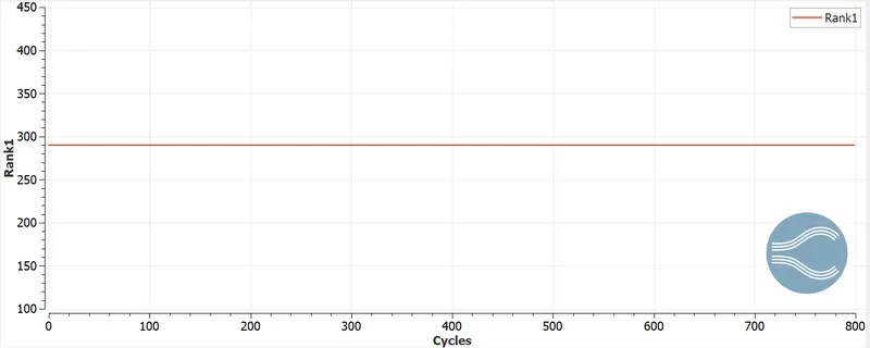
Transient flow:
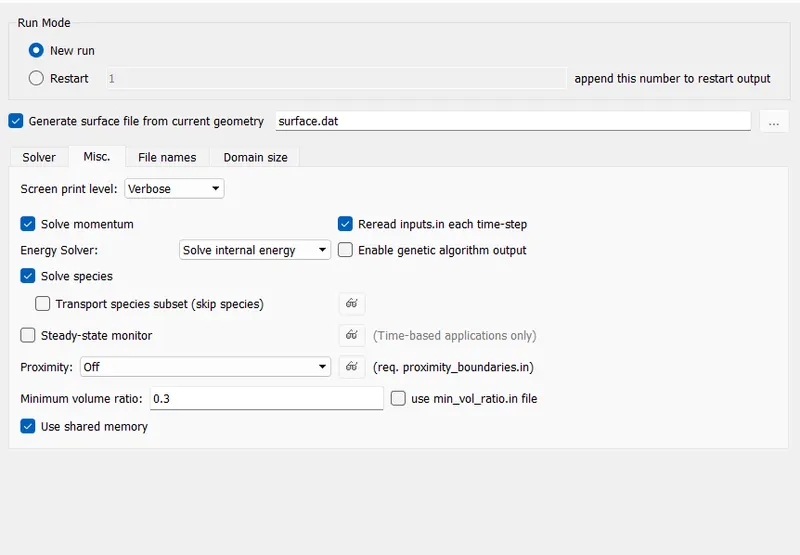
RANK Cycles:
Velocity Contour:
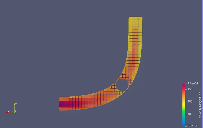
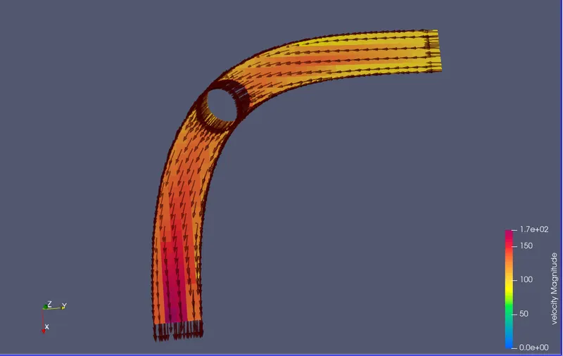
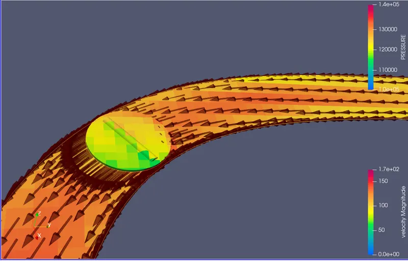
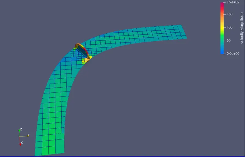
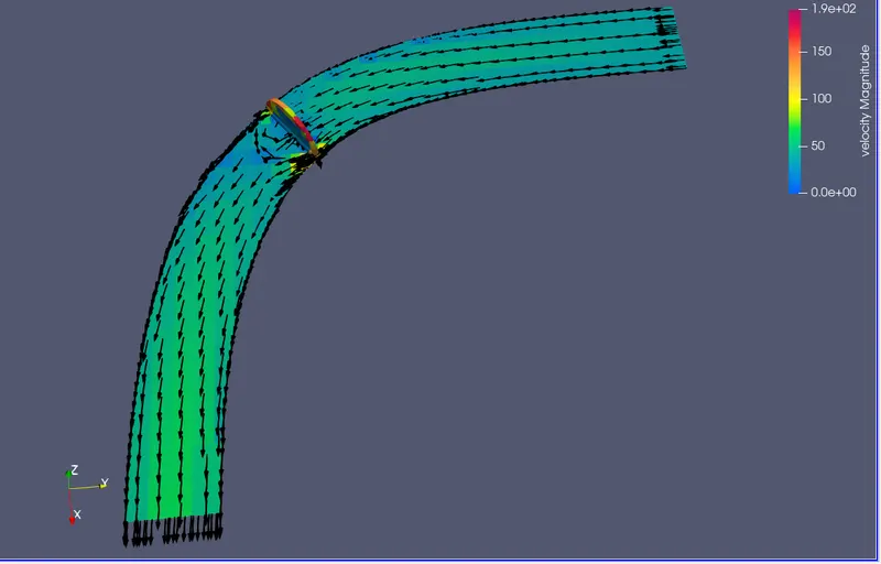
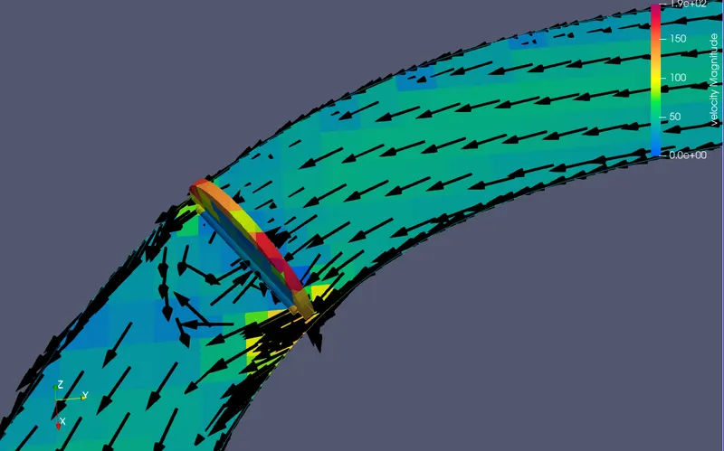
From figure eight, we will see the results of the varied rate across a throttle body. The accelerator is in a very wide-open position thanks to that the utmost quantity of fluid will meet up with that region from recess to outlet. however the throttle body still creates some disturbance because the minimum space of it's still in between the fluid path. thanks to this, there's a discount in fluid rate, the blue color shows the abrupt decrease in rate round the throttle edges wherever the fluid strikes kind the recess facet. because it passes over the throttle body, the highest and bottom portion of the throttle creates a slim path w.r.t elbow wall thanks to that there's a rise in rate then because the fluid fully passes over the throttle region it regains its original rate.
The average rate of flowing fluid in a very pipe is between 150-200 m/s with a scoop rate capable approx. three hundred m/s and min. rate capable approx. thirty m/s round the accelerator edges. the speed distribution round the accelerator will additional be clearly visible from figure nine i.e. from Stream-line rate contour.
Pressure Contour:
As we all know from the results of rate contour that once the fluid strikes down at the throttle body edges from the recess facet, its rate decreases. The pressure is reciprocally proportional to the speed and from figure ten (inlet side) we will see the utmost pressure at the region wherever the speed becomes minimum. Similarly, on the outlet facet, pressure decrease with the rise in rate.