Week 4.1: Project - Steady state simulation of flow over a throttle body

AIM:

To run the simulation for a steady state case of flow over a throttle body.

OBJECTIVE:

The main objective is to post process the results and show pressure and velocity conours.

To show the Mesh with surface with edges

Show the plots for pressure, velocity mass flow rate and total cell count.

Create an animation such that the throttle movement should be visible.

DESCRIPTION:

A throttle body is essentially a large air valve that sits between the intake manifold and the air intake pipe. An engine has one throttle body, which bolts to the intake manifold's plenum (the large air cavity in the center). A throttle body controls air flow into the engine, which crucial factor is for controlling the engine's air/fuel ratio. Throttle bodies comes in several shapes, sizes and configurations and can perform several tasks outside of their normal air-metering duties.

Throttle bodies usually use 'butterfly valves'. These valves consist of a casing with a large hole in the center, which is filled with a steel plate called as butterfly or throttle plate. The throttle shaft is a rod that passes through the housing and is connected to the throttle cable on the outside and the throttle plate on the inside. When the throttle shaft turns, it rotates the throttle plate, allowing air to go around it and into the engine.

STEADY STATE SIMULATION:

A staedy state simulation is used to investigate the steady state behaviour of a system, where the simulation continues until the system reaches a steady state.

Like in steady state mode, dynamic models are based on first principles that cannot be violated. Conservation laws, phase equilibrium, heat and mass transfer and kinetics are also applied in dynamic models. The most significant difference between a steady state and dynamic simulation is that steady state assumes that variables are constant with respect to time. This means in steady state there is no accumulation in the system. So the overall mass and energy input matches its output. Where as in dynamic models, consider the mass and energy rate of accumulation within the system, which allows one to determine how long does it would take to reach a stable condition starting from a specified initial state.

STEPS FOR RUNNING THE SIMULATION:

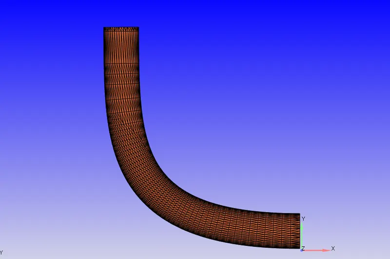
Opening the .stl model of elbow in the Converge studio as follows

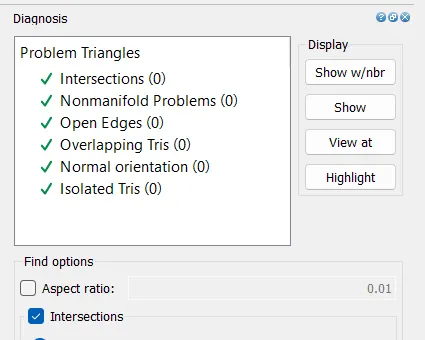
First checking up the diagonosis we see no errors

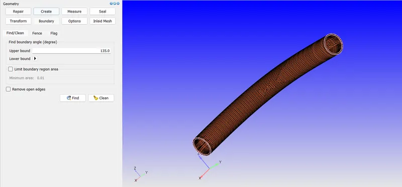
Creating boundary fence using Boundary>Find/clean as follows

As the geometry has some thickness to it, and we are not interested in heat transfer so we will delete the thickness of the elbow using Traingles by angle selection as follows

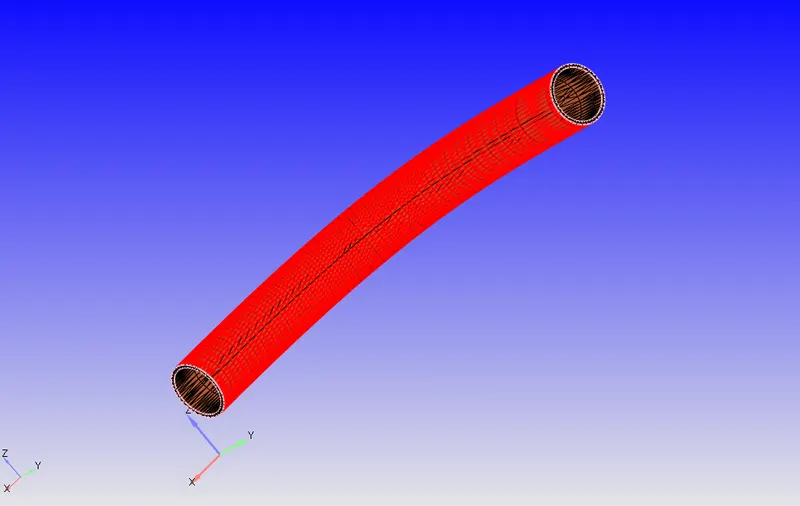
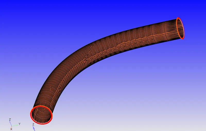
Now after deletion

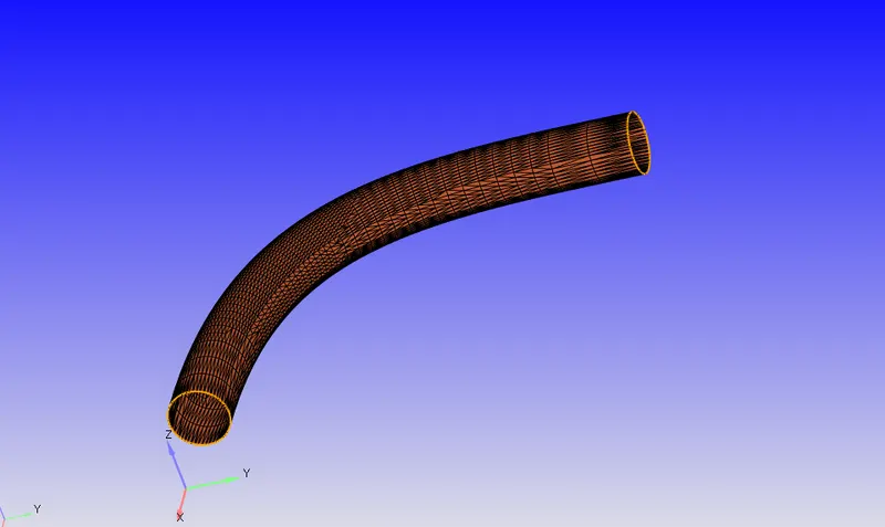
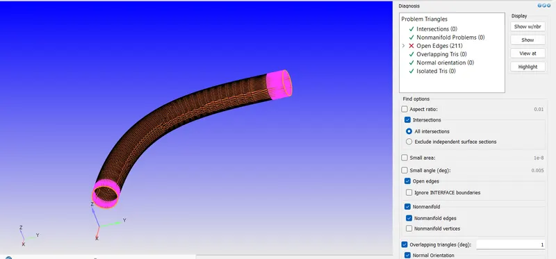
Now if we run the diagnosis we get the open edges error as there are in with yellow edge colour

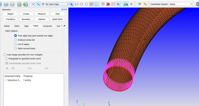
Using Repair>Patch with open edge selection we select and fill the openings

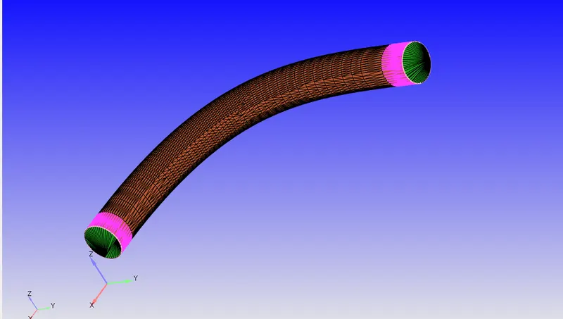
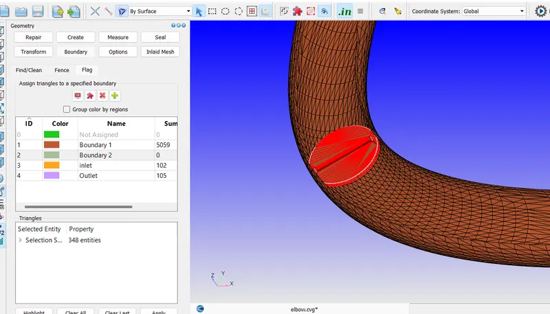
Assigning the boundaries using flagging

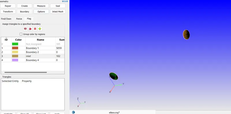
For inlet

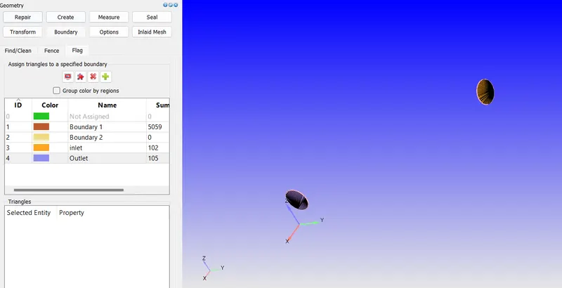
For outlet

Now hiding the part using Traingle any box selection to see the throttle

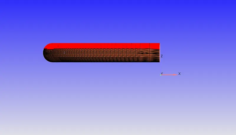
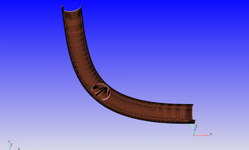
By using surface pick for throttle

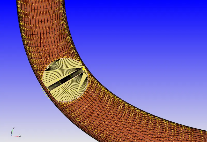
Now looking for normals we see they are pointing inwards which is correct as fuild flow is inside

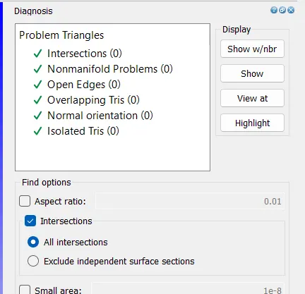
Now checking the diagnosis we see no errors

Now setting up the Case

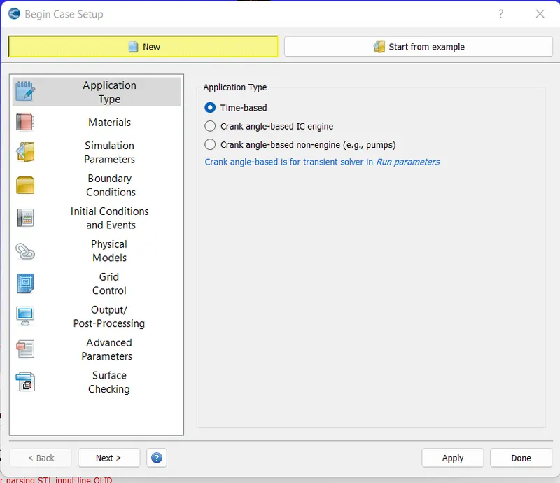
As we are doing the Non-reacting simulation we are not concerned with the IC engines so we select the time based

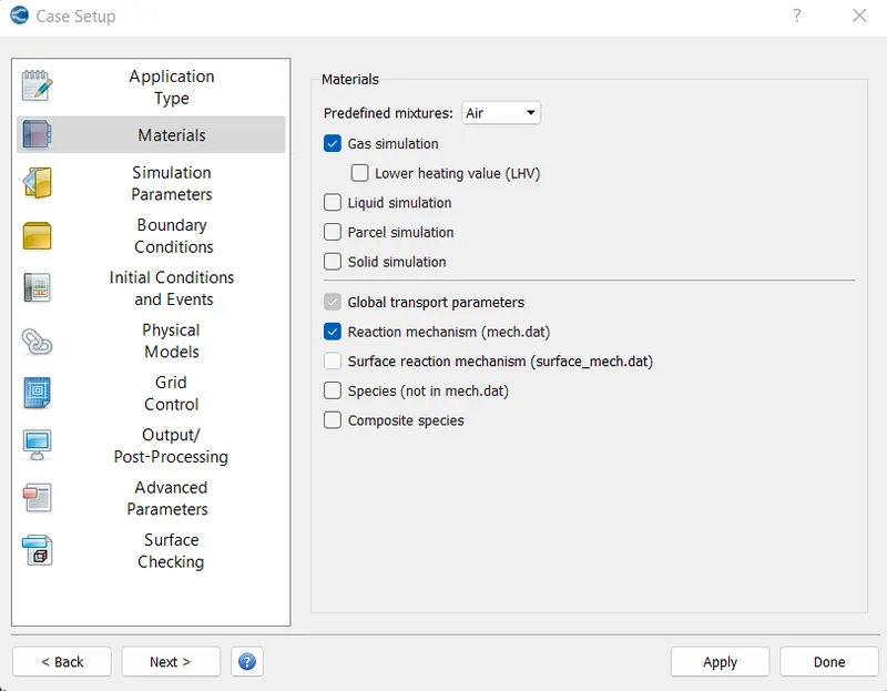
Simulating only for the gas flow so we select materials as Air

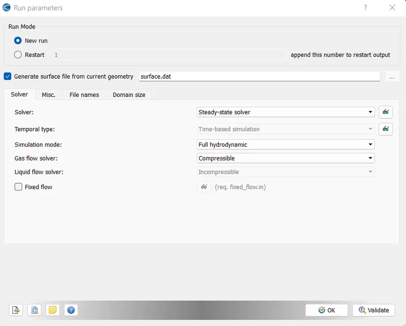
Now for run parameters as here valve is not moving we go for steady state solver

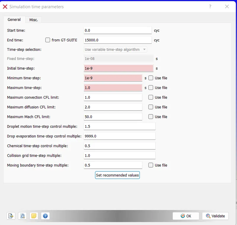
For simulation time parameters

And solver parameters- pressure based

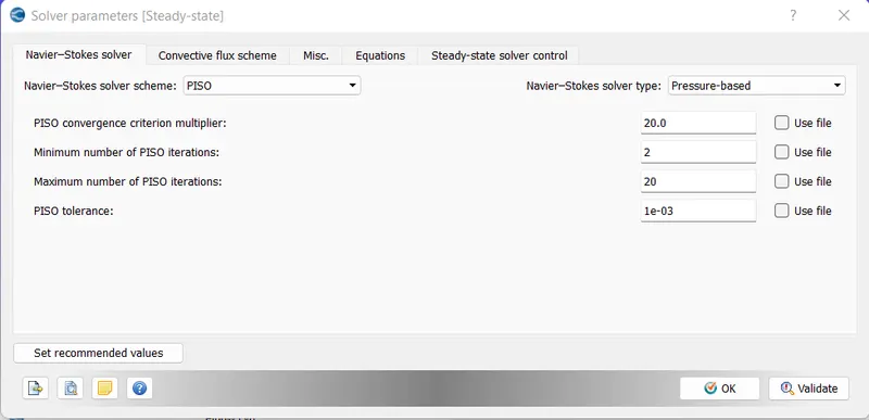
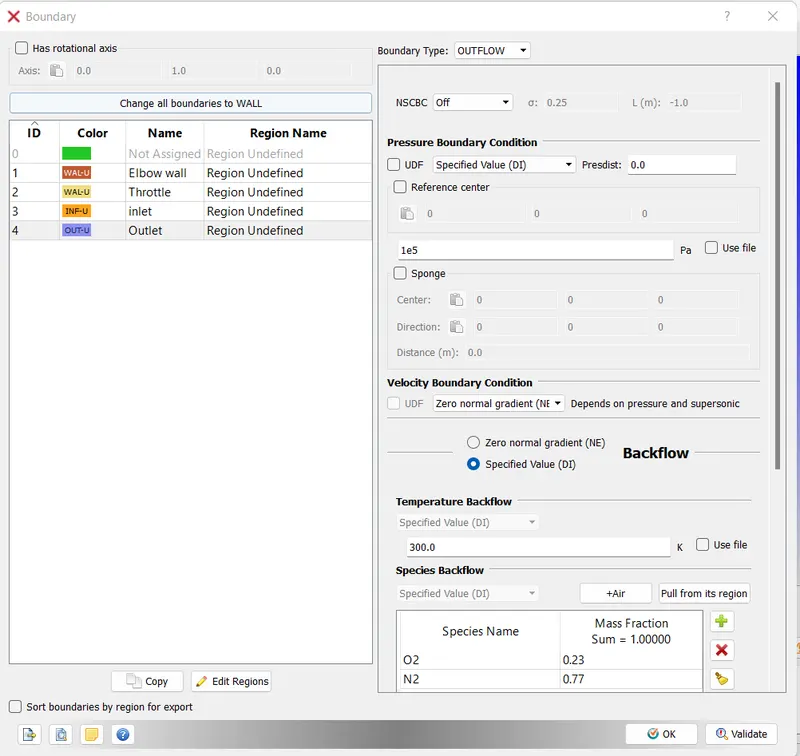
Now setting up the boundary

For elbow wall

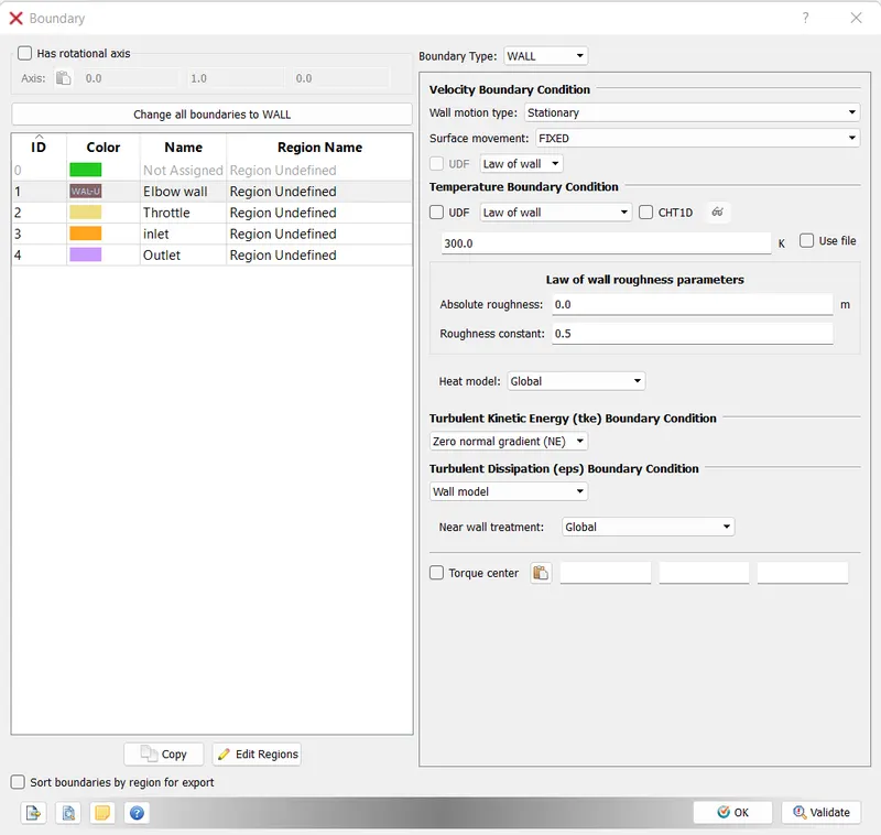
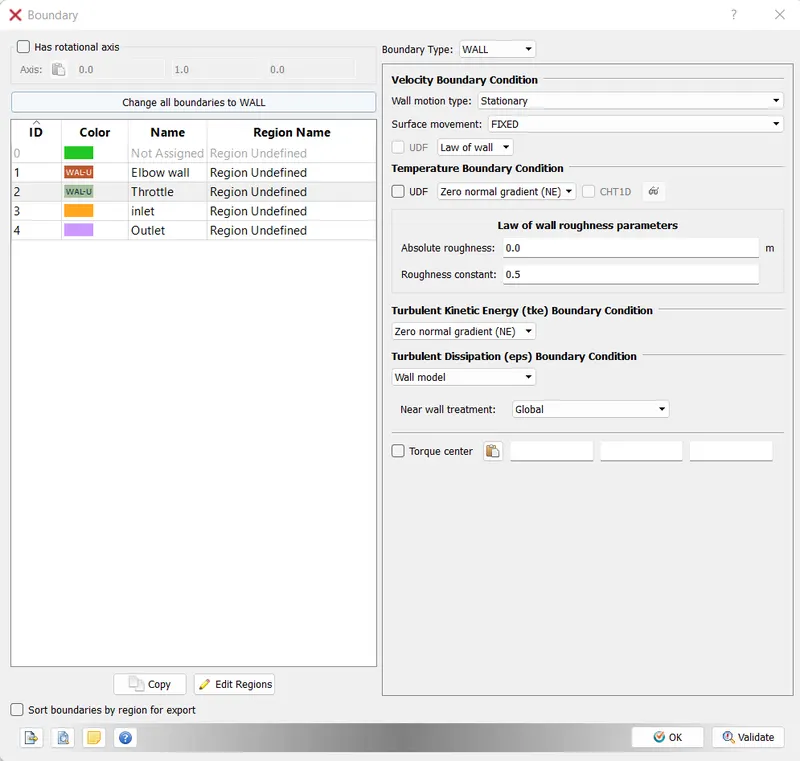
For throttle-for turbulent law of wall applies

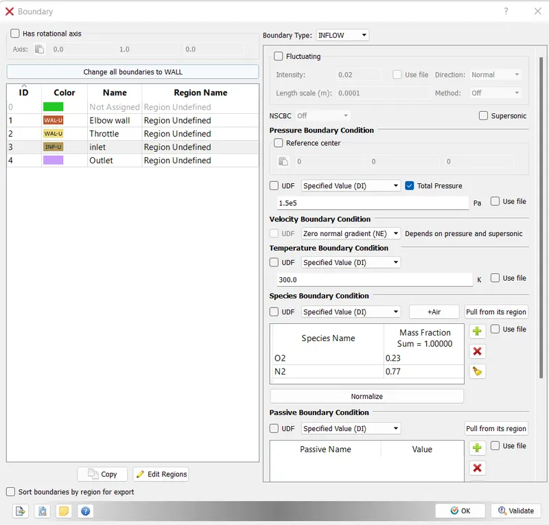
For inlet with inflow with 1.5bar pressure and with Air flow

For outlet, outflow with static pressure 1bar

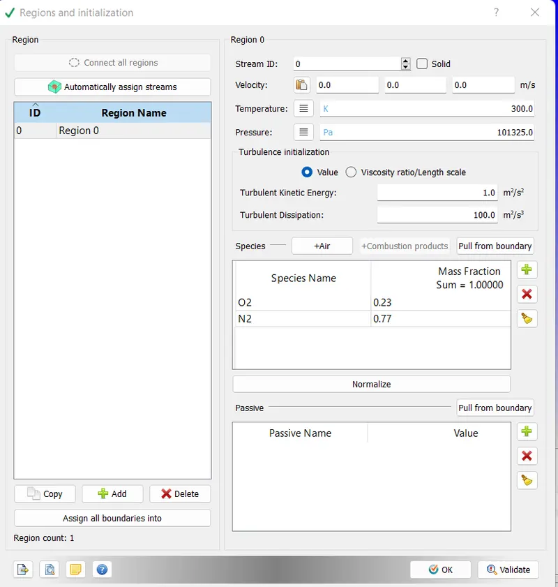
Now assigning the region

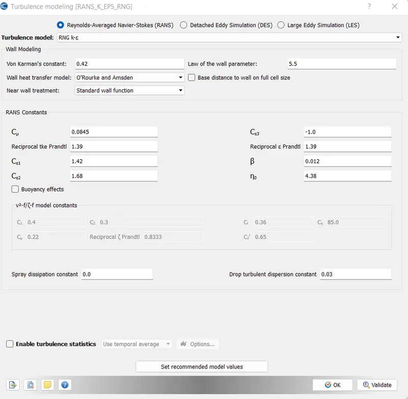
Turbulence model we go with RNG k-epsilon

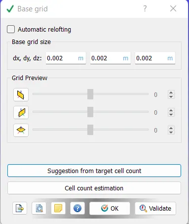
And we use 2mm base grid

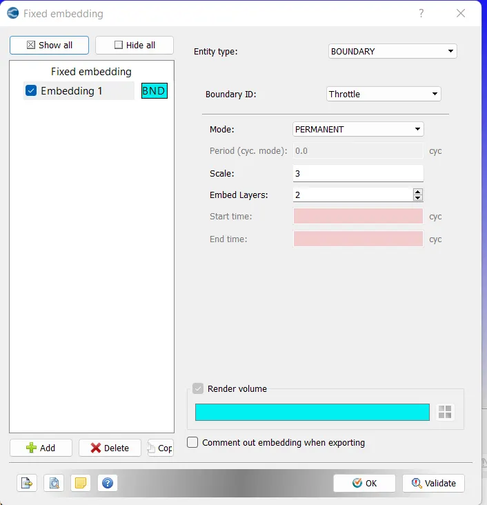
Fixed embedding

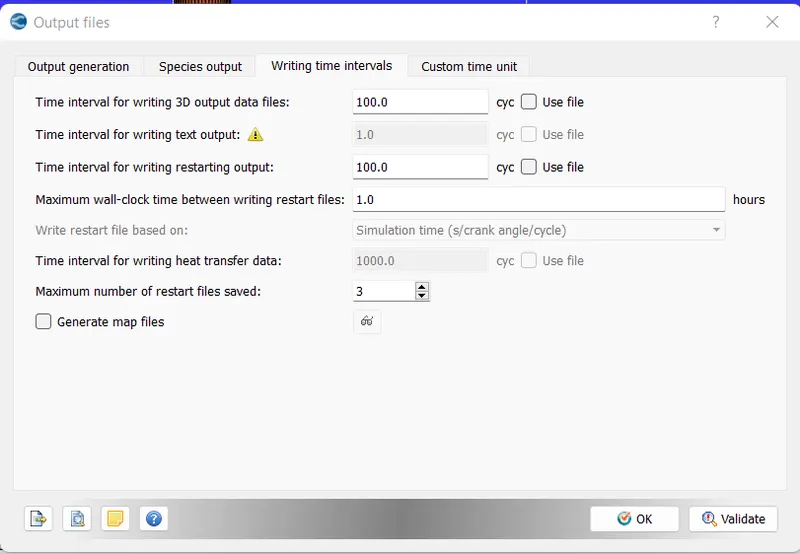
Output files

Then running the case set-up after exporting the input files to the folder using Cygwin.

By using the application mpiexec.exe & converge.exe by command line 'mpiexec.exe -n 2 converge.exe restricted' we run the simulation till results are converged.

Then using converge and paraview post processing results are observed and studied.

RESULTS:

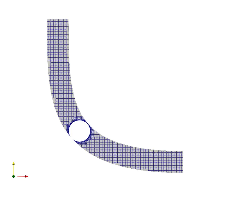
Mesh by using grid embedding

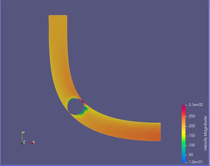
The velocity contours is

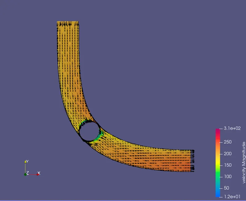
The velocity vectors are as follows

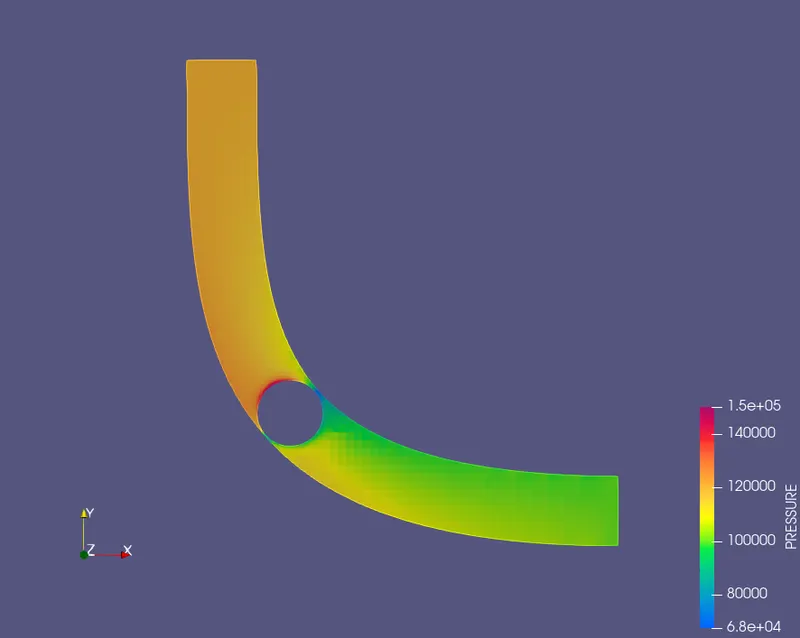
The pressure contours is

The throttle contour is

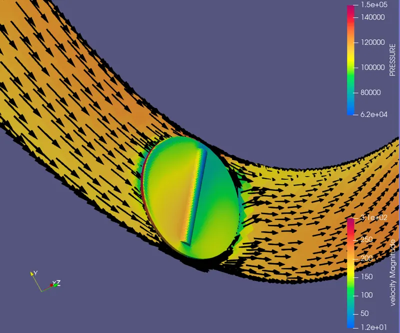
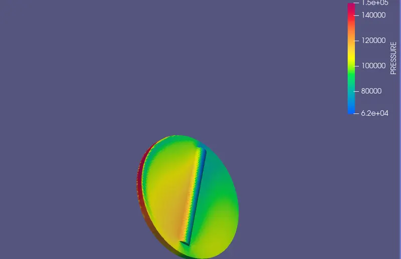
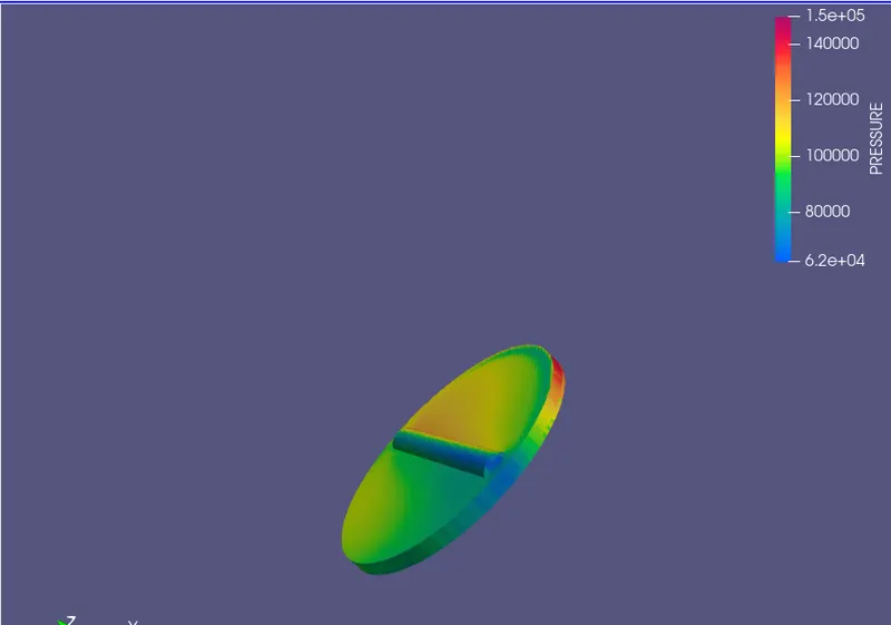
Here we see that at the start of throttle the pressure increases at the start and at the sides also some pressure can be seen.

The Animation is

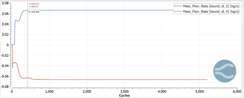
The Mass flow rate is

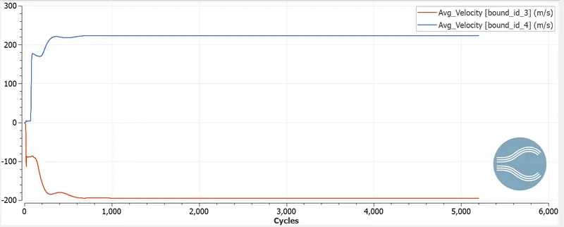
The velocity plots is

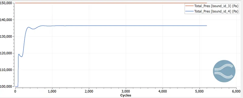
The total pressure is

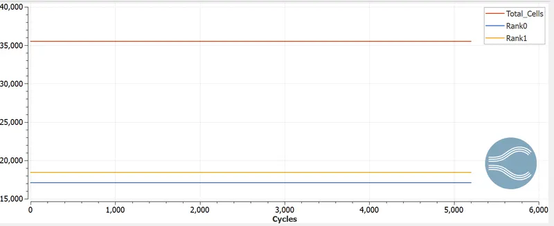
The cell count is

CONCLUSION:

Due to the fixed embedding of the throttle valve, the simulaions near to it become clear as the number of cell count is increases in the specified region.

The velocity increases near the elbow valve since the area is less and pressure gets dropped in the region which causes the velocity to increase.

The velocity of the fluid decreases when it collides with the throttle valve.

It also causes the formation of the stagnation point due to an increase in the pressure and decrease in the velocity.