Week 4.1 - Genetic Algorithm
Week 4.1 - Genetic Algorithm
AIM:
To create a Genetic Algorithm with a given staligmite function.
OBJECTIVES:
- Write a code in MATLAB to optimise the stalagmite function and find the global maxima of the function.
- Clearly expalin the concept of genetic algorithm in your own words and also explain the syntax for ga in MATLAB in your report.
- Make sure that your code gives the same output, even if it is made to run several times.
- Plot graphs for all 3 studies and for F maximum vs no. of iterations. Title and axes labels are a must, legends could be shown if necessary.
INTRODUCTION:
Genetic algorithm:It is a optimisation method which is based on Charls Darwins Theory of natural Evolution.evolution of natural selection is one of the most recogonised theory regarding natural selection,which also include geological refrences,genetics,environmantal factors and much more.
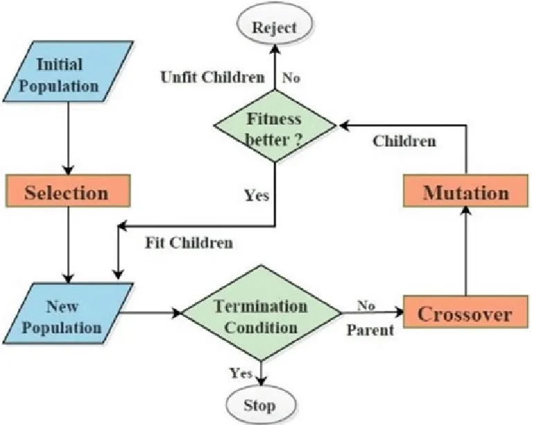
The genetic algorithm is a method for solving both constrained and unconstrained optimization problems that is based on natural selection, the process that drives biological evolution. The genetic algorithm repeatedly modifies a population of individual solutions. At each step, the genetic algorithm selects individuals from the current population to be parents and uses them to produce the children for the next generation. Over successive generations, the population "evolves" toward an optimal solution. You can apply the genetic algorithm to solve a variety of optimization problems that are not well suited for standard optimization algorithms, including problems in which the objective function is discontinuous, nondifferentiable, stochastic, or highly nonlinear. The genetic algorithm can address problems of mixed integer programming, where some components are restricted to be integer-valued.
-
Selection rules select the individuals, called parents, that contribute to the population at the next generation. The selection is generally stochastic, and can depend on the individuals' scores.
-
Crossover rules combine two parents to form children for the next generation.
-
Mutation rules apply random changes to individual parents to form children.
Advantages of ga:
- Is faster than most traditional methods.
- used to search from population of point and not single point
- Supports multi-objective optimisation
- Good for 'noisy' environment
- robust with respect to local maxima/minima
Disadvantage of ga:
- Not suited for all problrm,problems forwhich derivatives are available.
- Being stochastic there is no guarantee on optimalor quality of solution.
- If not implimented proprly, ga may not converge optimal solution.
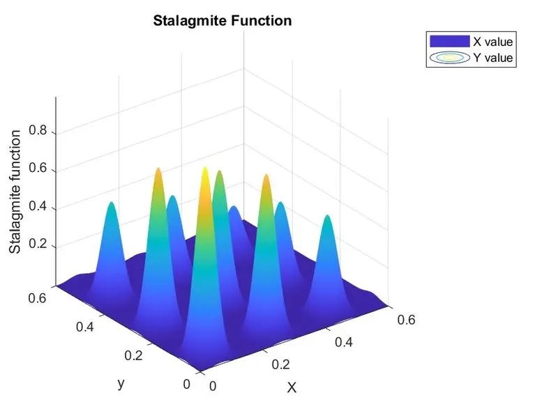
Stalagmite: A stalagmite is a type of rock formation that rises from the floor of a cave due to the accumulation of material deposited on the floor from ceiling drippings. Stalagmites are typically composed of calcium carbonate, but may consist of lava, mud, peat, pitch, sand, sinter, and amberat (crystallized urine of pack rats) . The graph obtained are similar shape to stalagmite.
Syntax:
x = ga( defines a set of lower and upper bounds on the design variables, fun,nvars,A,b,Aeq,beq,lb,ub)x, so that a solution is found in the range lb ≤ x ≤ ub. (Set Aeq=[] and beq=[] if no linear equalities exist.)
x = ga( subjects the minimization to the constraints defined in fun,nvars,A,b,Aeq,beq,lb,ub,nonlcon)nonlcon. The function nonlcon accepts x and returns vectors C and Ceq, representing the nonlinear inequalities and equalities respectively. ga minimizes the fun such that C(x) ≤ 0 and Ceq(x) = 0. (Set lb=[] and ub=[] if no bounds exist.)
x = ga( minimizes with the default optimization parameters replaced by values in fun,nvars,A,b,Aeq,beq,lb,ub,nonlcon,options)options. (Set nonlcon=[] if no nonlinear constraints exist.)
x = ga(fun,nvars,A,b,Aeq,beq,lb,ub,nonlcon,intcon,options)intcon take integer values.
[ also returns a matrix x,fval,exitflag,output,population,scores] = ga(___)population, whose rows are the final population, and a vector scores, the scores of the final population
STALAGMITE FUNCTION:
`f(x,y) = f_1 ,_x f_2,_x f_1 ,_y f_2,_y`
where,
`f_1,_x =[sin(5.1 pi x + 0.5)]^6`
`f_1,_y = [sin(5.1 pi y + 0.5)]^6`
`f_2,_x =exp[-4ln(2)(x-0.0667)^2/0.64]`
`f_2,_y =exp[-4ln(2)(y-0.0667)^2/0.64]`
CODE:
Function code:
Below given function code inputs the xand y vector from main loop and outputs staligmite output to the main code for optimisation. the function code is based on the equation above.
%creating a function to output staligmite variables
function [fxy]=stalagmite_func(input_vector)
%input_vector is split in 2 vectors x and y
    x=input_vector(1);
    y=input_vector(2);

    f1x=(sin(5.1*pi*x+ 0.5))^6;
    f1y=(sin(5.1*pi*y+ 0.5))^6;

    f2x=exp(-4*log(2)*(((x-0.0667)^2)/0.64));
    f2y=exp(-4*log(2)*(((y-0.0667)^2)/0.64));
%negative sign is multiplide to give is the inverse value of ga algorithm, as ga always provide minimum value
    fxy=-(f1x*f1y*f2x*f2y);
end
Maincode:
%Week 4.1 - Genetic Algorithm
%Write a code in MATLAB to optimise the stalagmite function and find the global maxima of the function.

clear all
close all
clc


 %define search space with maximum amd mimium value (x,y)axis
 x=linspace(0,0.6,150);
 y=linspace(0,0.6,150);
 %lowerbound for ga
 L_B=0;
 %upperbound for ga
 U_B=1;
 %creating a 2d mesh
 [xx,yy]=meshgrid(x,y);

% count be the number off iterations
count=55;

%start the clock
tic

%Evaluating the stalagmite function
%taking values for each  x and y
 for i=1:length(xx)
     for j=1:length(yy)
         input_vector(1)=xx(i,j);
         input_vector(2)=yy(i,j);
%        calling stalagmite_function
         f(i,j)=stalagmite_func(input_vector);
     end
 end

%ends the clock and saves time in variable study_time
study_time=toc

%create a new plot
figure(1)
%create a conture plot
surfc(xx,yy,-f)
%to remove refrence lines on the plot
shading interp
%label x,y, and z axis
xlabel('X')
ylabel('y')
zlabel('Stalagmite function')
%createe legent for plot term discription
legend('X value','Y value')
%create the title for figure
title('Stalagmite Function')
%save the figure1 as Stalagmite.jpeg injpeg format
saveas(1,'Stalagmite.jpeg')


%------------STUDY1----------- {unbounded condition}
%start timer
tic
% get ga value for 1 to 55 counts and store in vector fval ,vector xval ,
% vector yval
for i=1:count
    [inputs,fval1(i)]=ga(@stalagmite_func,2);
    xval1(i)=inputs(1);
    yval1(i)=inputs(2);
end
%end timer and stor in a variable
studytime1=toc
%create a new figure
figure(2)
%create a subplot for surfc gridrow-2, gridcoloum-1,posision-1
subplot(2,1,1)
surfc(x,y,-f)
%remove shading
shading interp
%add label, title and legend
xlabel('X')
ylabel('y')
zlabel('Stalagmite function')
title('Unbounded inputs')
legend('X value','Y value')
hold on
%plot marker on 3dplot
plot3(xval1,yval1,-fval1,'Marker','o','MarkerSize',5,'MarkerFaceColor','auto')
%second subplot to plot -fval1
subplot(2,1,2)
plot(-fval1)
%add label, title and legend
xlabel('iteration')
ylabel('Stalagmite function')
legend('optimal value')
%save the figure2 as Stalagmite.jpeg injpeg format
saveas(2,'unboundedga.jpeg')


%--------STUDY2---------{ga with upper and lower bound sampling}

%start timer
tic
% get ga value for 1 to 55 counts and store in vector fval ,vector xval ,
% vector yval
for i=1:count
    [inputs,fval2(i)]=ga(@stalagmite_func,2,[],[],[],[],[L_B;L_B],[U_B;U_B]);
    xval2(i)=inputs(1);
    yval2(i)=inputs(2);
end
%end timer and stor in a variable
studytime2=toc
%create a new figure
figure(3)
%create a subplot for surfc gridrow-2, gridcoloum-1,posision-1
subplot(2,1,1)
surfc(x,y,-f)
%remove shading
shading interp
%add label, title and legend
xlabel('X')
ylabel('y')
zlabel('Stalagmite function')
title('Bounded Inputs')
legend('X value','Y value')
hold on
%plot marker on 3dplot
plot3(xval2,yval2,-fval2,'Marker','o','MarkerSize',5,'MarkerFaceColor','auto')
%second subplot to plot -fval2
subplot(2,1,2)
plot(-fval2)
%add label, title and legend
xlabel('iteration')
ylabel('Stalagmite function')
legend('optimal value')
%save the figure3 as Stalagmite.jpeg injpeg format
saveas(3,'boundedga.jpeg')


%-------STUDY3-------{ga with upper and lower bound sampling and population size}
%asuume a population size of 200
%to add options.
options=optimoptions(@ga);
options=optimoptions(options,'PopulationSize',200);
%start timer
tic
% get ga value for 1 to 55 counts and store in vector fval ,vector xval ,
% vector yval
for i=1:count
    [inputs,fval3(i)]=ga(@stalagmite_func,2,[],[],[],[],[L_B;L_B],[U_B;U_B],[],[],options);
    xval3(i)=inputs(1);
    yval3(i)=inputs(2);
end
%end timer and stor in a variable
studytime3=toc
%create a new figure
figure(4)
%create a subplot for surfc gridrow-2, gridcoloum-1,posision-1
subplot(2,1,1)
surfc(x,y,-f)
%remove shading
shading interp
%add label, title and legend
xlabel('X')
ylabel('y')
zlabel('Stalagmite function')
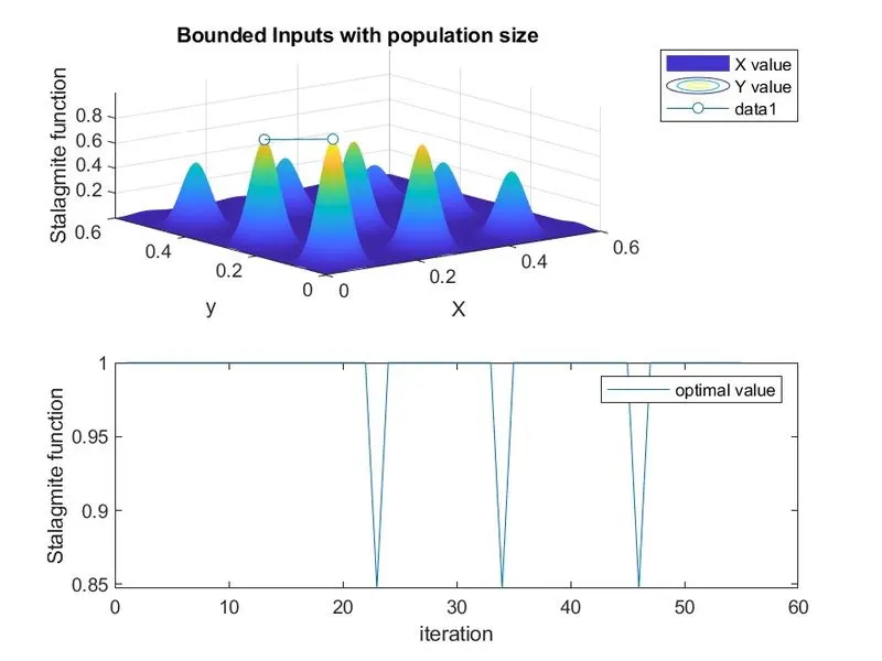
title('Bounded Inputs with population size')
legend('X value','Y value')
hold on
%plot marker on 3dplot
plot3(xval3,yval3,-fval3,'Marker','o','MarkerSize',5,'MarkerFaceColor','auto')
%second subplot to plot -fval3
subplot(2,1,2)
plot(-fval3)
%add label, title and legend
xlabel('iteration')
ylabel('Stalagmite function')
legend('optimal value')
%save the figure4 as Stalagmite.jpeg injpeg format
saveas(4,'boundewith_populationdga.jpeg')

%getting  global maxima with respect to study3
global_maxima=-fval3
code explenation:
initialy the we create a matrix for x and y value with a set of values,and few other variables that are requred for GA and iteration.
create a 2d mesh.
from the 2dmesh we take each individial value of x and y , put it in the stalagmite function code to output optimal function values as another vector.
A surface plot is genarated with axis x,y,z . z as staligmite function.labeling, title legend is added for clarity.
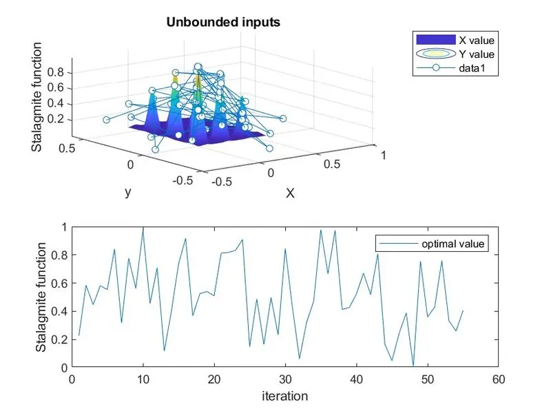
for study1 i.e., unbounded condition. random limits are generated.
ga function is called with just fuction and no of inputs, and this itterations are done 55 times .
graph is ploted with x,y, -functun.
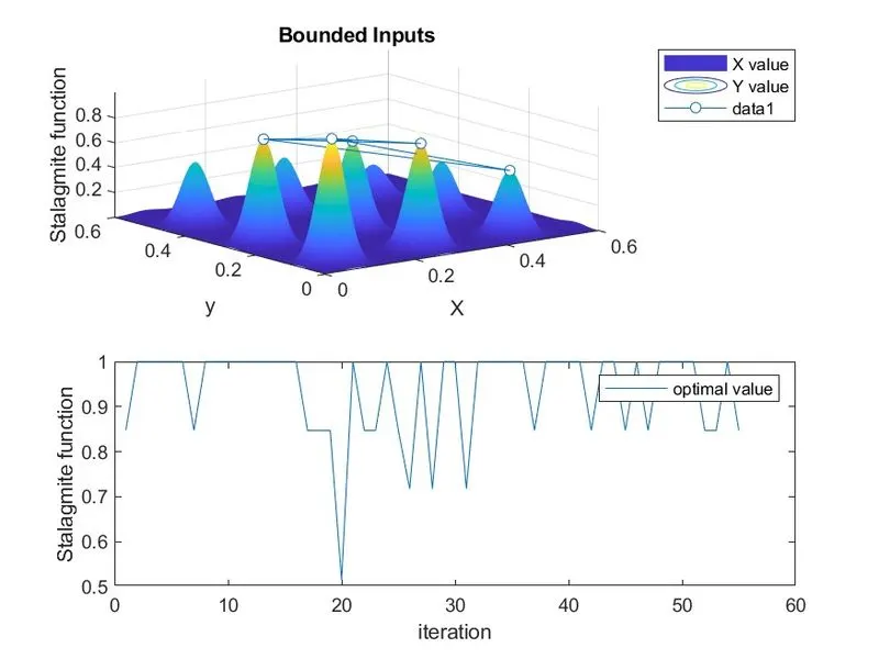
for study2 i.e., bounded condition. predefined values for upper and lover limit is set.
55 iterations are done with the syntax x = ga(fun,nvars,A,b,Aeq,beq,lb,ub)
two plots with surs=fc function on x,y,-fvalue is fenerated and also a plot with number of itteration and maxima.
for study3 i.e., bounded condition with poppulation. predefined values for upper and lover limit is set and population value.
x = ga(fun,nvars,A,b,Aeq,beq,lb,ub,nonlcon,intcon,options)
the above sintax is used to solve third part of problem
similar graph is made ,surfc function
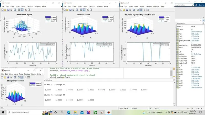
out put screenshots are provided below.
OUTPUTS:
STUDY1:
STUDY2:
STUDY 3:
REFRENCE:
https://in.mathworks.com/help/gads/what-is-the-genetic-algorithm.html
https://en.wikipedia.org/wiki/Genetic_algorithm