Week 4.1 - Genetic Algorithm

Step-wise explanation of code.

1.First, Linspace command is used to define x & y with 150 elements between zero and 0.6 including the bounds.Then num_cases is set which will be used as counter for iteration to 50

2.The 2D grid is made using meshgrid command is created from x & y input to be output to xx & yy after that for loop is used to solve the genetic algorithm for every element in the 2D mesh grid

3.The length of rows & column are used as counters the input vector is declared as ga requires input vector which is each value in the mesh grid then the output of stalagmite function is stored in matrix

4.the tic command is used to start a timer for loop bounded by the number of iterations is formed. The ga code is entered for unbounded statistical study which have the following

5. Then smallest (minimum) value of the function for each iteration is output & its x & y coordinates which are stored in seperate variables.the 'tic' command is used to stop the timer and the output is stored in study_time

6.The figurel is plotted by the following steps.First subplot command is used to partition the plot window in order to draw more than one plot in the same window, two rows and one column are specified and then the position of each plot is selected

7.Then hold on command is used to prevent plot for being removed.The surf command is used to plot contour with xx & y value from the mesh grid as input and negative optimum value is used because we need to maximize the function.then x,y,& z axis are labelled

8.The shading interp is used to smoothen the function plot and to remove the grid lines, plot 3 command is used to plot a point in 3D, here it will plot- fopt because we need the maximum value of the function not the minimum

9. then the graph title is selected. The opt value of the function is plotted on the second plot in the second row

10. Its x & y axis are labelled. Then the same study is made but this time it is bounded (has lower & upper limit) which requires the same commands and step excepts the ga command which have the following format:

input, fopt] = ga(fun, nvars, A, b, Aeq, beq, Ib, ub) Inputs, fopt, fun & nvars are the same as study-l
A - Linear inequality constraints : real matrix, if
there are none, then[]
b- Linear inequality constraints : real vector, if there are none, then []
Aeq - Linear equality constraints - :- real matrix, if
there are none, then []
beq - Linear equality constraints - real vector, if
there are none, then[]
Ib - lower bounds, specified as a real vector or
array
ub - upper bounds, specified as a real vector or
array

11. The range of the genetic algorithm is bounded by introducing values for lower and upper bounds and hence the values of global maxima and the values of × & y will be within the defined search space in inputs

12. then increasing population size study was done which is the same as before but it had different ga code of :
and study -2 respectivelly nonlcon - nonlinear constraints, specified as a function handle or function name. If there are none then IntCon - Integer variables, specified as a vector of positive integers, if there are none, then [] Options - Optimization options, specified as the output of optimoptions or a structure.

13. The range of the genetic algorithm is bounded as in study-2 but to improve the accuracy, the commands optimoptions is introduced to increase the Population Size,total time is computed.then using fprintf command the results are printed in the command windows

14. Then the study time is printed. the x, y coordinate of the maximum optimum values are printed

15. The optimum values of the function (maximum value) is printed which is calculated from the (negative mean) of the all iterations of the output value and the negative sign is used to get the maximum value

16. Then the study time of the whole 3 studies combined is printed.

MATLAB CODE:

1)STALAGMITE FUNCTION

clear all
close all
clc


% Defining our search space
x = linspace(0,0.6,150);
y = linspace(0,0.6,150);
num_case = 60;

% Creating a 2 dimensional mesh
[xx,yy] = meshgrid(x,y);

% Evalutting the stalagmite function

for i = 1:length(xx)
    for j = 1:length(yy)
        input_vector (1) = xx(i,j);
        input_vector (2) = yy(i,j);
        f(i,j) = stalagmite (input_vector);
    end
end

tic
for k = 1:num_case
    [inp,favl(k)]=  ga(@stalagmite,2);
    x_1 (k) = inp(1);
    y_1 (k) = inp(2);
end

figure (1)
hold on
grid on
surfc(xx,yy,-f)
shading interp
title('stalagmite plot')
xlabel ('X' )
ylabel("y")

figure (2)
subplot (2,1,1)
surfc(xx,yy,-f)
shading interp
hold on
plot3(x_1,y_1,-favl, 'marker', 'o', 'markersize',5,'markerfacecolor','g')
title('unbounded inputs')
subplot (2,1,2)
plot(-favl)
xlabel('iterations')
ylabel('function minimum')

FUNCTION FILE:

function [f] = stalagmite(input)
x = input (1);
y = input (2) ;
f1x = (sin (5.1*pi*x + 0.5)) ^6;
f1y = (sin(5.1*pi*y + 0.5)) ^6;
f2x = exp((-2.7726)*(x-(0.0667))^2/0.64);
f2y = exp((-2.7726)*(y- (0.0667)) ^2/0.64) ;
f= -(f1x*f1y*f2x*f2y) ;
end

RESULT for basic stalagmite function and

CASE STUDY(|)

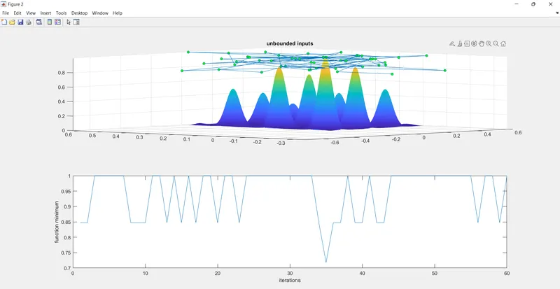
Here,in the case study(1), the solutions are not bounded so the GA will calculated all the possible maximima in'x' and 'y' coordinates. and the time taken to calculates the possibile solution is 4.4339

CASE STUDY (||)

MATLAB CODE:

clear all
close all
clc


% Defining our search space
x = linspace(0,0.6,150);
y = linspace(0,0.6,150);
num_case = 60;

% Creating a 2 dimensional mesh
[xx,yy] = meshgrid(x,y);

% Evalutting the stalagmite function

for i = 1:length(xx)
    for j = 1:length(yy)
        input_vector (1) = xx(i,j);
        input_vector (2) = yy(i,j);
        f(i,j) = stalagmite (input_vector);
    end
end


tic
for s = 1:num_case;
[input, fval(s)]= ga(@stalagmite, 2,[],[],[],[],[0,0],[0.6,0.6]);
x_2 (s) = input(1) ;
y_2(s) = input(2);
end
study2_time = toc

figure(3)
subplot (2,1,1)
surfc(xx,yy,-f)
shading interp
hold on
plot3(x_2,y_2,-fval, 'marker', 'o', 'markersize',5,'MarkerFaceColor','g')
title(' unbounded inputs')
subplot (2,1,2)
plot(-fval)
xlabel('iterations')
ylabel('function minimum')

RESULT:

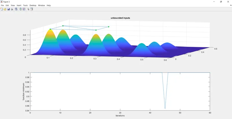
As we can see that the time taken in result two studies is 6.1952 for the reading of global maxima. Here, are using genetic algorithm tool to bound the lower and upper value, because when we bound the upper and lower value then the ga tool will search in that range only. here, the lower and upper bound are taken as (0 and .6) for the x and y-direction.

CASE STUDY (|||)

MATLAB CODE:

clear all
close all
clc


% Defining our search space
x = linspace(0,0.6,150);
y = linspace(0,0.6,150);
num_case = 60;

% Creating a 2 dimensional mesh
[xx,yy] = meshgrid(x,y);

% Evalutting the stalagmite function

for i = 1:length(xx)
    for j = 1:length(yy)
        input_vector (1) = xx(i,j);
        input_vector (2) = yy(i,j);
        f(i,j) = stalagmite (input_vector);
    end
end

% 3rd case study increasing ga iteration
options = optimoptions('ga');
options = optimoptions (options, 'PopulationSize',150);
tic
for m = 1: num_case;
[input, fval(m)]= ga(@stalagmite, 2,[],[],[],[],[0,0],[0.6,0.6],[],[],options);
x_3 (m) = input (1) ;
y_3 (m) = input (2) ;
end

study3_time = toc
figure(4)
subplot (2,1,1)
surfc(xx,yy,-f)
shading interp
hold on
plot3 (x_3,y_3,-fval, 'marker', 'o', 'MarkerSize',5,'MarkerFaceColor','g')
title(' unbounded inputs')
subplot(2,1,2)
plot(-fval)
xlabel('iterations')
ylabel('function minimum')

RESULT:

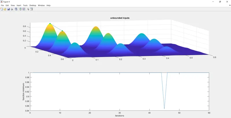
The resulted line from high peak to low peak is the critical point for my global maxima and the time taken by it is 36.4559 which is approx 3 times greater than the case study one. As the population size is large enough to carry out 50 iterations at the same time. however, we got our optimum maximized solution.

MATLAB FINAL CODE FOR ALL THREE STUDIES:

clear all
close all
clc


% Defining our search space
x = linspace(0,0.6,150);
y = linspace(0,0.6,150);
num_case = 60;

% Creating a 2 dimensional mesh
[xx,yy] = meshgrid(x,y);

% Evalutting the stalagmite function

for i = 1:length(xx)
    for j = 1:length(yy)
        input_vector (1) = xx(i,j);
        input_vector (2) = yy(i,j);
        f(i,j) = stalagmite (input_vector);
    end
end

tic
for k = 1:num_case
    [inp,favl(k)]=  ga(@stalagmite,2);
    x_1 (k) = inp(1);
    y_1 (k) = inp(2);
end
study1_time=toc

tic
for s = 1:num_case;
[input, favl(s)] = ga(@stalagmite,2,[],[],[],[],[0,0],[0.6,0.6]);
x_2 (s) = input(1) ;
y_2(s) = input(2);
end
study2_time = toc

% 3rd case study increasing ga iteration
options = optimoptions('ga');
options = optimoptions (options, 'PopulationSize',150);
tic
for m = 1: num_case;
[input,fval(m)]= ga(@stalagmite, 2,[],[],[],[],[0,0],[0.6,0.6],[],[],options);
x_3 (m) = input (1) ;
y_3 (m) = input (2) ;
end

study3_time = toc

figure (1)
hold on
grid on
surfc(xx,yy,-f)
shading interp
title('stalagmite plot')
xlabel ('X' )
ylabel('y')

figure (2)
subplot (2,1,1)
surfc(xx,yy,-f)
shading interp
hold on
plot3(x_1,y_1,-favl,'marker','o','markersize',5,'markerfacecolor','g')
title('unbounded inputs')
subplot (2,1,2)
plot(-favl)
xlabel('iterations')
ylabel('function minimum')

%2nd case study statistical behaviour

figure(3)
subplot (2,1,1)
surfc(xx,yy,-f)
shading interp
hold on
plot3(x_2,y_2,-fval, 'marker', 'o', 'markersize',5,'MarkerFaceColor','g')
title(' unbounded inputs')
subplot (2,1,2)
plot(-fval)
xlabel('iterations')
ylabel('function minimum')

%3rd case increasing ga iterations

figure(4)
subplot (2,1,1)
surfc(xx,yy,-f)
shading interp
hold on
plot3 (x_3,y_3,-fval, 'marker', 'o', 'MarkerSize',5,'MarkerFaceColor','g')
title(' unbounded inputs')
subplot(2,1,2)
plot(-fval)
xlabel('iterations')
ylabel('function minimum')

In many problems, GAs have a tendency to converge towards local optima or even arbitrary points rather than the global optimum of the problem. This means that it does not "know-how" to sacrifice short-term fitness to gain longer-term fitness. we may come out from this problem by using a different fitness function, increasing the rate of mutation, or by using selection techniques that maintain a diverse population of solutions. we can not trust genetic algorithms because Diversity is important in genetic algorithms or genetic programming because crossing over a homogeneous population does not yield new solutions. In evolution strategies and evolutionary
programming, diversity is not essential because of a greater reliance on mutation.

ERROR WHILE PROGRAMMING:

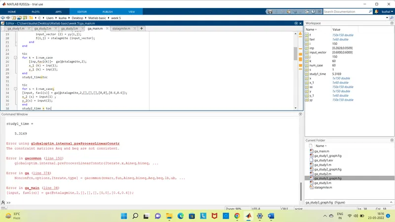
The error was in the GA algorithm syntax, wherein i did not type '[]'.