Week 4.1 - Genetic Algorithm

Aim

• Write a code in MATLAB to optimise the stalagmite function and find the global maxima of the function.
• Plot graphs for all 3 studies and for F maximum vs no. of iterations. Title and axes labels are a must, legends could be shown if necessary.

Introduction

The global maxima of a 'Stalagmite Function' can be obtained using 'Genetic Algorithm' in MATLAB.

Genetic algorithms are a class of algorithms based on the abstraction of Darwin's evolution of biological systems, pioneered by Holland. He was probably the first to use genetic operators such as the crossover and recombination, mutation, and selection in the study of adaptive and artificial systems. Three main components or genetic operators in genetic algorithms are

• Mutation

• Selection of the fittest.

• Crossover

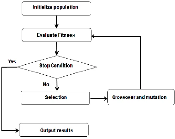
The genetic algorithm can be applied to solve a variety of optimization problems that are not well suited for standard optimization algorithms, including problems in which the objective function is discontinuous, nondifferentiable, stochastic, or highly nonlinear.

Function Defined

 %stalagmite function with input as input_vector which contains the

function [f]= stalagmite(input_vector)
x= input_vector(1);

y= input_vector(2);

f1= (sin(5.1*pi*x+0.5))^6; 
f2= (sin(5.1*pi*y+0.5))^6;
f3= exp(-4*log(2)*(x-0.0667)^2/0.64); 
f4= exp(-4*log(2)*(y-0.0667)^2/0.64);
f= -(f1*f2*f3*f4); % The Negative sign denotes he inverse of the Stalagmite function and is added in order

end

Where,

x is the local minima point.

fun is the function to be called. (In our case, its the stalagmite function)

nvars indicates the no of variables used. 4. A and b are used to indicate any kind inequalities that exist in the function.

Aeq and Beq also denotes the inequalities.

lb = lower bound.

ub = upper bound.

nonicon gives a two vectors representing inequalities and equalities.

options is used to perform additional operations like increasing population size. This is done with the help of "optimoptions".

Final Code

clear all
close all
clc

% x and y inputs

x=linspace (0,0.6,150);
y= linspace(0,0.6,150); 
[xx,yy]= meshgrid(x,y);

for i=1:length(xx)
     for j= 1:length(yy)
         input_vector(1) = xx(i,j);
         input_vector(2) = yy(i,j);
         f(i,j)=stalagmite(input_vector);

     end
end


num_cases=150; % GA runs for 150 iterations
options= optimoptions('ga');
options= optimoptions (options, 'PopulationSize',450);

tic % Study Time start

for i=1:num_cases

% Objective function is stalagmite and the number of varaibles is 21

% A, B, Aeq and Beq = [], as there is no Linear equalities and inequalities constraints in this function % lower boundary of varaibles x and y in ga alogorithmn is set as [0,0]

% upper boundary of varaibles x and y in ga alogorithmn is set as [0.6,0.6] % population size is defined by using options in the algorithmn

[inputs,f_opt(i)]= ga(@stalagmite,2,[],[],[],[],[0,0],[0.6,0.6],[],options);
x_opt(i)=inputs(1);
y_opt(i)=inputs(2); 
opt_f(i)= -f_opt(i); %Ga gives us Minima value. Inverse f_opt is taken for Maxima value. 
end

Study3_time = toc % Study Time end 
subplot(2,1,1)
hold on

surfc(xx, yy, f) %Generating the stalagmite function. 
shading interp % To bring visually smooth curve surface without mesh lines 
plot3(x_opt,y_opt,f_opt,'marker','o','markersize',5,'markerfacecolor','r') 
title('Bounded inputs with increased population size')
subplot(2,1,2) 
plot(opt_f) %Plotting opt_f value for every iteration
xlabel('Number of iterations ---->') 
ylabel('Function Max -->')

Final Output

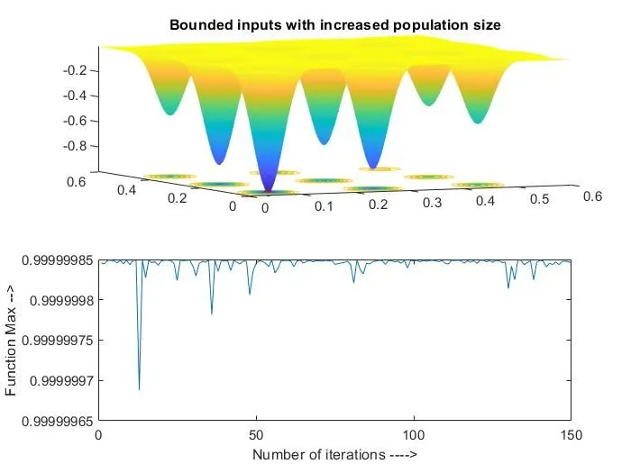
EXPLANATION OF PROGRAM:

Initially, the stalagmite function was mentioned with appropriate argument vectors.

• The program has been subdivided into three studies based on the limitations of the previous study.

• First study deals with unbounded inputs, thereby expanding the boundary wherein the results can be obtained.

• Second study brings in the aspect of bounded inputs providing a better solution for the drawback faced.

• Third study lays a appreciable platform to determine the exact solution.

• Plots of all the three studies have been displayed, thus giving a clear insight of the results.

CONCLUSION:

The Global Maxima is calculated by Population Sizing and the plots provide a visual context of the solution and verifies the authenticity of the obtained value.