Week 3 - Solving second order ODEs

Objective:

Write a program that solves the following ODE. This ODE represents the equation of motion of a simple pendulum with damping

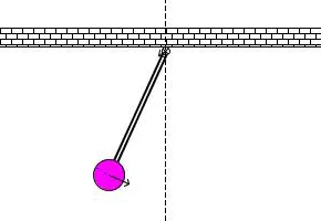
When you do this you will get the position of the pendulum as a function of time. Use this information to animate the motion of the pendulum, as shown in the below figure.

Introduction

For a pendulum swinging back and forth, the amount of time required to complete one full
swing is called the period. that the period depends only on the length
of the pendulum and the acceleration due to gravity. In fact, the period and the length of
the pendulum are related by a power function. In this lab we will establish the relationship
between the period and the length of the pendulum by measuring the period for differing
lengths.

Given Data

In the above equation,

g = gravity in m/s2,

L = length of the pendulum in m,

m = mass of the ball in kg,

b=damping coefficient.

Write a program in Matlab\Octave that will simulate the pendulum motion, just like the one shown in the start of this challenge.

use,

L=1 metre,

m=1 kg,

b=0.05.

g=9.81 m/s2.

Simulate the motion between 0-20 sec,

for angular displacement=0,

angular velocity=3 rad/sec at time t=0.

Matlab Program

function [dtheta_dt] = ode_func(t,theta,b,g,l,m)

theta1 = theta(1)
theta2 = theta(2)
dtheta1_dt = theta2;
dtheta2_dt = -(b/m)*theta2 - (g/1)*sin(theta1);
dtheta_dt = [dtheta1_dt; dtheta2-dt];
end
close all
clear all
clc
%inputs
b= 0.05;
g =9.81;
l = 1;
m = 1;

%initial Condition
theta_0 = [0 5];

%time point
time_span = linspace(0,10,100);

%solving ODE
[t,results] = ode45(@(t,theta) ode_func(t,theta,b,g,l,m),time_span,theta_0);
figure(1);
plot(t,[results(:,1) results(:,2)])
ylabel('plot')
xlabel('time')

theta = results(:,1);
c = 1

for i = 1:length(theta)
    Theta = theta(i);
    
    %initial point
    x0 = 0;
    y0 = 0;
    
    %movement of pendulum
    x1 = 1*sin(Theta);
    y1 = -1*cos(Theta);
    
    figure (2);
    %plotting sting
    plot([x0 x1],[y0 y1],'color','g');
    hold on
    0%plotting pendulum bob
    plot(x1,y1,'O','markersize',10,'color','r','MarkerFaceColor','r');
    hold off
    
    axis([-1 1 -1.5 0]);
    pause(0.03);
    M(c) = getframe(gcf);
    c = c+1;
end
% making a movie
movie(M);
videofile = VideoWriter('ODE.avi','Uncompressed avi');
open(videofile)
writeVideo(videofile,M)
close(videofile)

Final Output

Conclusion

We Have understood How to solve Second Order ODE Using Matlab.