Week 4.1 - Genetic Algorithm
Generic Algorithm
Objective:
- To optimise the stalagmite function and find the global maxima of the function using Generic Algorithm.
- Generic algorithm repeatedly modifies a population of individual solutions. At each step, the genetic algorithm randomly selects individuals from the current population and uses them as parents to produce the children for the next generation. Over successive generations, the population "evolves" toward an optimal solution.
- Optimizing the values is the main objective of this program.
Program:
#these commands are used to clear the command window and the workspace so that new values will be used
clear all
close all
clc
% Stalagmite Mathematical model
# the space defined should be smaller so that the generic algorithm works accurately and the optimization will be obtained
% Defining the search space
#linspace is used to keep the values constant between two numbers taken and assigned for x & y values
x = linspace(0,0.7,180);
y = linspace(0,0.7,180);
[xx,yy] = meshgrid(x,y);
% Stalagmite function
for i = 1:length(xx)
for j = 1:length(yy)
inputs(1) = xx(i,j);
inputs(2) = yy(i,j);
# Stalagamite command is used to find the local and global maxima for the given values
f(i,j) = stalagmite(inputs);
end
end
# num_case - is used to get the optimization for 50 times.
num_case = 50;
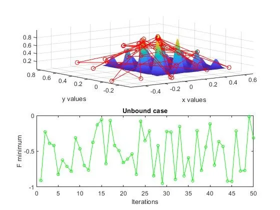
# Case 1 - The boundary values is not set and the optimization takes place without boundary values.
% Stalagmite without bound case - Study 1
# tic and toc is used to record the current time and elasped time respectively.
tic
for k = 1:num_case
[inputs,f_opt(k)] = ga(@stalagmite,2);
x_opt(k) = inputs(1);
y_opt(k) = inputs(2);
end
toc
% Plotting without bound
figure(1)
#sub plot is used to two graphs in a single figure by splitting the figure window
subplot(2,1,1);
# surfc is used for 3d plotting with contour plot
surfc(x,y,-f);
# shading interp is used for making smooth curves without grid lines
shading interp
hold on;
xlabel('x values');
ylabel('y values');
# plot3 is used to plot in 3d space
plot3(x_opt,y_opt,-f_opt,'Marker','o','Color','r');
subplot(2,1,2);
plot(f_opt,'Marker','o','MarkerSize',4,'Color','g');
title('Unbound case');
xlabel('Iterations');
ylabel('F minimum');
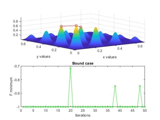
# Case 2 - The boundary values is not set and the optimization takes place with boundary values.
% Stalagmite with bound case - Study 2
tic
for m = 1:num_case
# Ga function is modified by giving the lower bound and upper bound values
[inputs,f_opt(m)] = ga(@stalagmite,2,[],[],[],[],[0;0],[0.4;0.4]);
x_opt(m) = inputs(1);
y_opt(m) = inputs(2);
end
toc
% Plotting
figure(2)
subplot(2,1,1);
surfc(x,y,-f);
shading interp
hold on;
xlabel('x values');
ylabel('y values');
plot3(x_opt,y_opt,-f_opt,'Marker','o','Color','r');
subplot(2,1,2);
plot(f_opt,'Marker','o','MarkerSize',4,'Color','g');
title('Bound case');
xlabel('Iterations');
ylabel('F minimum');
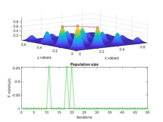
Case 3 - The boundary values is not set and the optimization takes place with boundary values and increasing the population size
% Stalagmmite bound and changing population size - Study 3
# This is used to give the population size values
options = optimoptions('ga');
options = optimoptions(options,'PopulationSize',200);
tic
for n = 1:num_case
[inputs,f_opt(n)] = ga(@stalagmite,2,[],[],[],[],[0;0],[0.4;0.4],[],[]);
x_opt(n) = inputs(1);
y_opt(n) = inputs(2);
end
toc
% Plotting
figure(3)
subplot(2,1,1);
surfc(x,y,-f);
shading interp
hold on;
xlabel('x values');
ylabel('y values');
plot3(x_opt,y_opt,-f_opt,'Marker','o','Color','r');
subplot(2,1,2);
plot(f_opt,'Marker','o','MarkerSize',4,'Color','g');
title('Population size');
xlabel('Iterations');
ylabel('F minimum');
Output : The optimization is good when when we give bound values and changing the population size.
clear all
close all
clc

% Stalagmite Mathematical model

% Defining the search space
x = linspace(0,0.7,180);
y = linspace(0,0.7,180);
[xx,yy] = meshgrid(x,y);

% Stalagmite function
for i = 1:length(xx)
    for j = 1:length(yy)
        inputs(1) = xx(i,j);
        inputs(2) = yy(i,j);
        f(i,j) = stalagmite(inputs);
    end
end

num_case = 50;

% Stalagmite without bound case - Study 1
tic
for k = 1:num_case
    [inputs,f_opt(k)] = ga(@stalagmite,2);
    x_opt(k) = inputs(1);
    y_opt(k) = inputs(2);
end
toc


% Plotting without bound
figure(1)
subplot(2,1,1);

surfc(x,y,-f);
shading interp
hold on;
xlabel('x values');
ylabel('y values');

plot3(x_opt,y_opt,-f_opt,'Marker','o','Color','r');
subplot(2,1,2);
plot(f_opt,'Marker','o','MarkerSize',4,'Color','g');
title('Unbound case');
xlabel('Iterations');
ylabel('F minimum');

% Stalagmite with bound case - Study 2
tic
for m = 1:num_case
    [inputs,f_opt(m)] = ga(@stalagmite,2,[],[],[],[],[0;0],[0.4;0.4]);
    x_opt(m) = inputs(1);
    y_opt(m) = inputs(2);
end
toc

% Plotting
figure(2)
subplot(2,1,1);
surfc(x,y,-f);
shading interp
hold on;
xlabel('x values');
ylabel('y values');


plot3(x_opt,y_opt,-f_opt,'Marker','o','Color','r');
subplot(2,1,2);
plot(f_opt,'Marker','o','MarkerSize',4,'Color','g');
title('Bound case');
xlabel('Iterations');
ylabel('F minimum');

% Stalagmmite bound and changing population size - Study 3

options = optimoptions('ga');
options = optimoptions(options,'PopulationSize',200);
tic
for n = 1:num_case
    [inputs,f_opt(n)] = ga(@stalagmite,2,[],[],[],[],[0;0],[0.4;0.4],[],[]);
    x_opt(n) = inputs(1);
    y_opt(n) = inputs(2);
end
toc

% Plotting
figure(3)
subplot(2,1,1);
surfc(x,y,-f);
shading interp
hold on;
xlabel('x values');
ylabel('y values');


plot3(x_opt,y_opt,-f_opt,'Marker','o','Color','r');
subplot(2,1,2);
plot(f_opt,'Marker','o','MarkerSize',4,'Color','g');
title('Population size');
xlabel('Iterations');
ylabel('F minimum');