Week 4.1 - Genetic Algorithm
Aim: - Write a matlab code to optimize the stalagmite function
Objectives: -
- Write a code in MATLAB to optimise the stalagmite function and find the global maxima of the function.
- Expalin the concept of genetic algorithm in and also explain the syntax for ga in MATLAB.
- Plot graphs for all 3 studies and for F maximum vs no. of iterations.
Introduction to Genetic Algorithm
Genetic algorithm is a search-based optimization technique based on the principles of Genetics and Natural selection. It is frequently used to find optimal solutions to both constrained and unconstrained problems. The genetic algorithm repeatedly modifies a population of individuals solutions. At each step, the genetic algorithm selects individuals from the current population to be parents and uses them to produce the children for the next generation. Over successive generations, the population “evolves” towards an optimal solution. Some examples of GA applications are optimizing decision trees for better performance, solving sudoku puzzles, hyperparameter optimization etc.
The flow chart shows the main algorithmic steps involved.
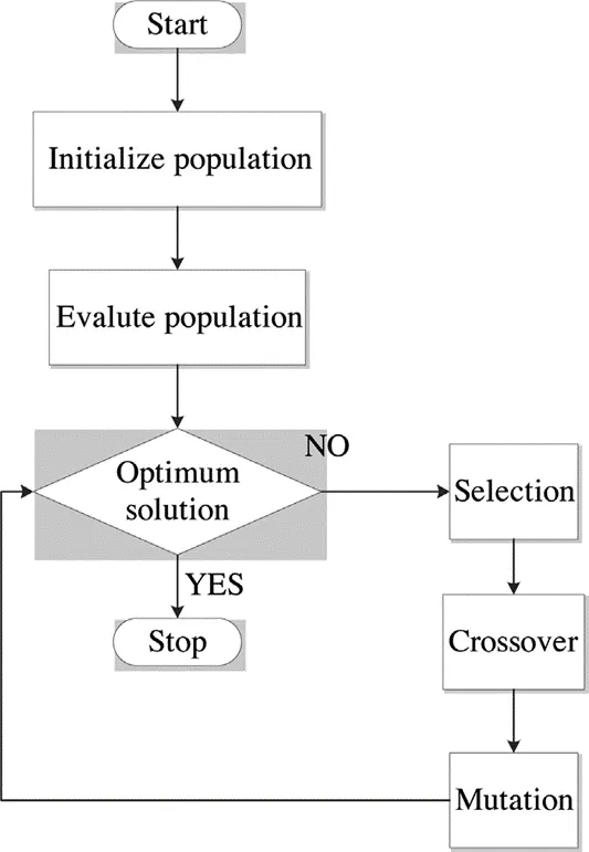
Initialization: - After the genetic representation and the fitness function are defined, a GA proceeds to initialize a population of solutions. The population size depends on the nature of the problem, but typically contains several hundreds or thousands of possible solutions.
Selection: - During each successive generation, a portion of the existing population is selected to breed a new generation. Individual solutions are selected through a fitness-based process, where fitter solutions are typically more likely to be selected. Certain selection methods rate the fitness of each solution and preferentially select the best solutions.
Crossover and mutation: - It is the process of producing a second-generation population of solutions from those selected. By producing a child solution using the methods of crossover and mutation, a new solution is created which typically shares many of the characteristics of its parents. New parents are selected for each new child, and the process continues until a new population of solutions of appropriate size is generated.
Syntax for GA algorithm
The syntax used in this program are as follows: -
x = ga(fun,nvars,A,b,Aeq,beq,lb,ub)
x = ga(fun,nvars,A,b,Aeq,beq,lb,ub,nonlcon,intcon,options)
x = ga(fun,nvars) finds a local unconstrained minimum, x, to the objective function, fun. nvars is the dimension (number of design variables) of fun.
x = ga(fun,nvars,A,b,Aeq,beq,lb,ub) defines a set of lower and upper bounds on the design variables, x, so that a solution is found in the range lb ≤ x ≤ ub. When there is no linear inequalities we set Aeq and Beq as null vector.
x = ga(fun,nvars,A,b,Aeq,beq,lb,ub,nonlcon,options) minimizes with the default optimization parameters replaced by values in options. (Set nonlcon=[] if no nonlinear constraints exist.) we Create options using optimoptions.
Stalagmite function
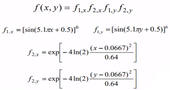
Stalagmite is a type of rock formation that rises from the floor of a cave due to the accumulation of material deposited on the floor from ceiling drippings. Stalagmite function is the mathematical function which generates similar shapes to stalagmites. Stalagmite function is a two-variable function, mathematically it is represented as: -
Code for stalagmite function
function [f] = stalagmite(input_vector)
f1x = (sin((5.1*pi).*input_vector(1)+0.5)).^6;
f1y = (sin((5.1*pi).*input_vector(2)+0.5)).^6;

f2x = exp((((input_vector(1)-0.0667).^2)/0.64).*(-4*log(2)));
f2y = exp((((input_vector(2)-0.0667).^2)/0.64).*(-4*log(2)));
f1=f1x*f1y*f2x*f2y;
f=-f1;
end
Main code for optimization
%Creating the search space to be optimized
%one dimensional

clear all
close all
clc
n=150;
x = linspace(0,0.6,150);
y = linspace(0,0.6,150);
tic

%creating two dimensional grid
[xx, yy] = meshgrid(x,y);

%evaluating the stalagmite function

for i = 1:length(xx)
    for j = 1:length(yy)
        input_vector(1)= xx(i,j);
        input_vector(2)= yy(i,j);
        f(i,j) = stalagmite(input_vector);
    end
end

figure(1)
surfc(xx, yy, f)
shading interp
xlabel('x value');
ylabel('y value');
study_time=toc;

%case 1 (unbounded inputs)
tic
for i = 1:n
    [inputs,fopt(i)]= ga(@stalagmite, 2);
    xopt(i)=inputs(1);
    yopt(i)=inputs(2);
end
figure(2)
subplot(2,1,1)
hold on
surfc (x,y,-f)
shading interp
plot3(xopt,yopt,-fopt,'marker','o','markersize',5,'markerfacecolor','r')
title('unbounded inputs')
subplot(2,1,2)
plot(-fopt)
xlabel('no. of iterations');
ylabel('function max');
study_time1=toc;

% second case (bounded inputs)
tic
for i = 1:n
    [inputs,fopt(i)]= ga(@stalagmite, 2,[],[],[],[],[0;0],[0.6;0.6]);
    xopt(i)=inputs(1);
    yopt(i)=inputs(2);
end
figure(3)
subplot(2,1,1)
hold on
surfc (x,y,-f)
shading interp
plot3(xopt,yopt,-fopt,'marker','o','markersize',5,'markerfacecolor','r')
title('bounded inputs')
subplot(2,1,2)
plot(-fopt)
xlabel('no. of iterations');
ylabel('function max');
study_time2=toc;

% third case (bounded inputs with increased population)

tic
options=optimoptions('ga');
options=optimoptions(options,'PopulationSize',500);

for i = 1:n
    [inputs,fopt(i)]= ga(@stalagmite,2,[],[],[],[],[0;0],[1;1],[],[],options);
    xopt(i)=inputs(1);
    yopt(i)=inputs(2);
end
figure(4)
subplot(2,1,1)
hold on
surfc (x,y,-f)
shading interp
plot3(xopt,yopt,-fopt,'marker','o','markersize',5,'markerfacecolor','r')
title('bounded inputs with increases population')
subplot(2,1,2)
plot(-fopt)
xlabel('no. of iterations');
ylabel('function max');
study_time3=toc;
Stepwise explanation of the program
- Program starts with clear all, close all, and clc. These commands clear the workspace area and closes all the figures.
- Firstly, search space has been defined using the linspace command, and meshgrid command is used to create the 2d array.
- A sub program is created to evaluate stalagmite function and result is stored in f variable.
- Figure 1 is plotted to show the 3d representation of stalagmite function.
Case study 1 – Statistical behaviour (unbounded)
- Ga solver is iterated for 150 times, and in this case no limits are provided.
- Ga solver returns two outputs, one is the minimum function value and other is the coordinates of the minimum value. Minimum value of function is stored in fopt(i) and coordinates are stored in xopt and yopt. This loop is run for 150 times and results are plotted.
- Figure 2 holds two plots, one showing the 3d representation of stalagmite with optimization results and other showing the function value.
- Plot3 command is used toplot a set of coordinates connected by line segments.
- Tic and toc command is used to monitor the time taken to complete the iterations.
- There is no upper and lower limit provided, hence algorithm is searching outside the search space.
Case study 2 – bounded inputs
- In the second case ga solver is run with upper and lower limits. This narrows down the search space and it becomes easier for the solver to find global minima.
- Four null vectors are passed in the solver syntax because there is no linear inequality involved in the stalagmite function.
- Again, the loop is run for 150 times and results are plotted in figure 3.
Case study 3 – bounded inputs with increased population size
- In the third case the solver is run with the bounded inputs along with the increased population size.
- PopulationSize specifies how many individuals are there in each generation. With a large population size, the genetic algorithm searches the solution space more thoroughly, thereby reducing the chance that the algorithm returns a local minimum that is not a global minimum. However, a large population size also causes the algorithm to run more slowly.
- Optimoptions command is used to create optimization options.
- options= optimoptions(SolverName) returns a set of default options for the SolverName
Results and discussion
1) Plot for stalagmite function
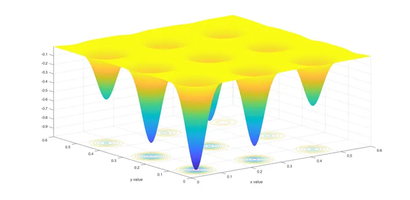
The above plot shows the 3d representation of stalagmite function. A function named stalagmite has been created to evaluate the mathematical expression and store the result in the form of an array. surfc(X,Y,Z) has been used to create a three-dimensional surface plot with a contour plot underneath.
2) Plot for unbounded inputs
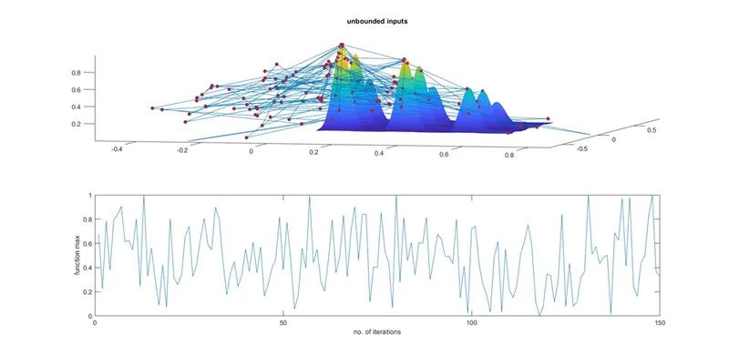
As from the above plot it can be observed that with the unbounded inputs ga solver is unable to calculate the global maxima. Due to random sampling the maximum value ranges between 0.1 to 1, hence further optimization is needed.
3) Plot for bounded inputs
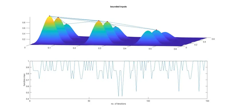
The above plot shows that using the bounded inputs gets more clear result than the previous one. Here the maximum value ranges between 0.7 to 1. But still optimization is needed.
4) Plot for bounded inputs with increased population size
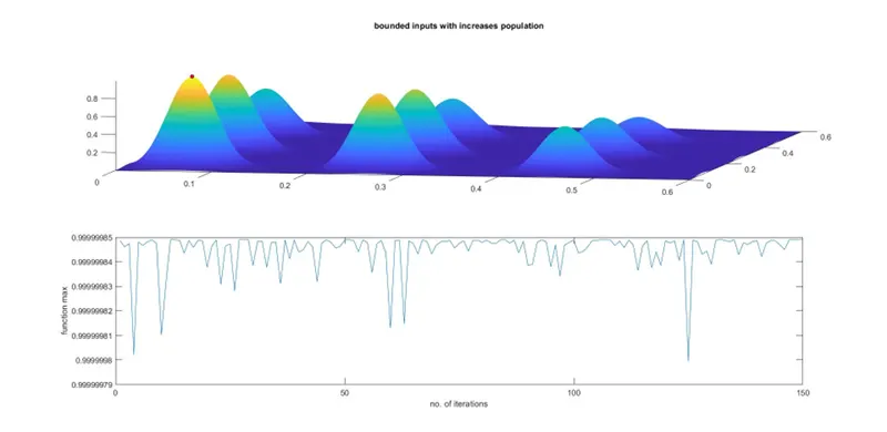
With the increased population size we get the most accurate result which is in between 0.99999983 to 0.99999985.
Error faced while writing the program

there was a syntax error which was resolved by correctly applying the optimoptions syntax.
Conclusions: -
- The ga solver is an inbuilt algorithm in matlab for optimization problem.
- Using the solver with bounded inputs gets more accurate results.
- The maximum value of the function lies between 0.99999983 to 0.99999985.
References: -
- wikipedia.org/wiki/Stalagmite
- mathworks.com/help/gads/genetic-algorithm-options.html
- Matlab help documentation