Week 4.1 - Genetic Algorithm

Theory for Genetic Algorithm

A genetic algorithm is an adaptive heuristic search algorithm inspired by "Darwin's theory of evolution in Nature."

The genetic algorithm is a method for solving both constrained and unconstrained optimization problems that is based on natural selection, the process that drives biological evolution. The genetic algorithm repeatedly modifies a population of individual solutions. At each step, the genetic algorithm selects individuals from the current population to be parents and uses them to produce the children for the next generation. Over successive generations, the population "evolves" toward an optimal solution.

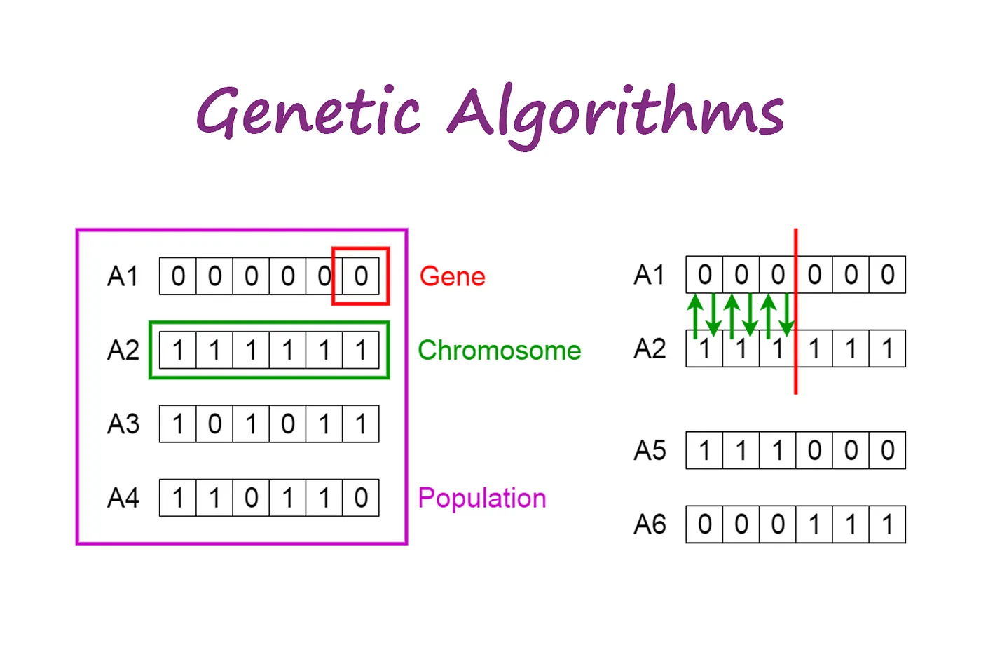
Notion of Genetic Algorithm

The process of natural selection starts with the selection of fittest individuals from a population. They produce offspring which inherit the characteristics of the parents and will be added to the next generation. If parents have better fitness, their offspring will be better than parents and have a better chance at surviving. This process keeps on iterating and at the end, a generation with the fittest individuals will be found.

This notion can be applied for a search problem. We consider a set of solutions for a problem and select the set of best ones out of them.

Five phases are considered in a genetic algorithm.

1. Initial population
2. Fitness function
3. Selection
4. Crossover
5. Mutation

1. Initial Population

A population of people is the starting point of the procedure. Every person is a component of the answer to the issue you're trying to address.

Genes are a set of parameters (variables) that define an individual. A chromosome is made up of a string of genes (solution). A string, or an alphabet, is used in a genetic algorithm to represent a person's collection of genes. Binary values are typically used (string of 1s and 0s). We refer to the genes on a chromosome as being encoded.

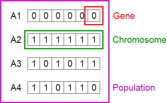
2. Fitness Selection

The fitness function determines how fit an individual is (the ability of an individual to compete with other individuals). It gives a fitness score to each individual. The probability that an individual will be selected for reproduction is based on its fitness score.

3. Selection

The idea of selection phase is to select the fittest individuals and let them pass their genes to the next generation.

Two pairs of individuals (parents) are selected based on their fitness scores. Individuals with high fitness have more chance to be selected for reproduction.

4.Crossover

Crossover is the most significant phase in a genetic algorithm. For each pair of parents to be mated, a crossover point is chosen at random from within the genes.

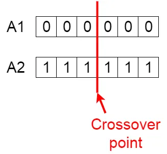
5. Mutation

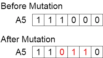
Mutation occurss to maintain diversity within the population and prevent premature convergence.

Equations used

The function used is for the genetic algorithm of the global maxima. we've taken the '-' of the function to attain the maxima value.

Process

1. Starting up with stalagmite function

2. Evaluating Stalagmite

3. Coding for unbounded input

4. Coding for bounded input

5. Coding for bounded input with modified population size

Coding for stalagmite function

function [f]=get_stalagmite(input_vector)

f1=(sin(5.1*pi*input_vector(1)+0.5))^6;
f2=(sin(5.1*pi*input_vector(2)+0.5))^6;
f3=exp(-4*log(2)*((input_vector(1)-0.0667)^2)/0.64);
f4=exp(-4*log(2)*((input_vector(2)-0.0667)^2)/0.64);
f= -(f1*f2*f3*f4);
end

Code for all three studies

clear all
close all
clc
x = linspace(0,0.6,150);
y = linspace(0,0.6,150);
[xx,yy] = meshgrid(x,y);
num_cases = 20;
for i = 1:length(xx)
    for j= 1:length(yy)
        input_vector(1)=xx(i,j);
        input_vector(2)=yy(i,j);
        f(i,j)= get_stalagmite(input_vector);
    end
end

for i = 1:num_cases
    [inputs, fopt(i)] = ga(@get_stalagmite, 2);
    xopt(i) = inputs(1);
    yopt(i) = inputs(2);
end
fopt=-fopt;
figure(1)
subplot(2,1,1)

surfc(x,y,-f)
shading interp
hold on
plot3(xopt,yopt,fopt,'marker','o','markersize',5,'markerfacecolor','r')
title('Unbounded inputs')
subplot(2,1,2)
plot(fopt)
xlabel('Iterations')
ylabel('Function minimum')
tic
%Study 2 -Statistical behavior - with upper and lower bound
for i = 1:num_cases
[inputs2, fopt2(i)] = ga(@get_stalagmite, 2,[],[],[],[],[0;0],[0.4;0.4]);
xopt2(i) = inputs2(1);
yopt2(i) = inputs2(2);
end
fopt2 = -fopt2;
study2_time = toc;
figure(2)
subplot(2,1,1)

surfc(x,y,-f)
shading interp
hold on
plot3(xopt2,yopt2,fopt2,'marker','o','markersize',5,'markerfacecolor','r')
title('bounded inputs')
subplot(2,1,2)
plot(fopt2)
xlabel('Iterations')
ylabel('Function minimum')
% Study 3 increasing GA iterations
options = optimoptions('ga');
options = optimoptions(options,'populationsize',200);
tic
for i = 1:num_cases
   [inputs3, fopt3(i)] = ga(@get_stalagmite,2,[],[],[],[],[0;0],[0.4;0.4],[],[],options);
    xopt3(i) = inputs3(1);
    yopt3(i) = inputs3(2);
end
study3_time = toc
figure(3)
subplot(2,1,1)

surfc(x,y,-f)
shading interp
hold on
plot3(xopt3,yopt3,-fopt3,'marker','o','markersize',5,'markerfacecolor','r')
title('bounded inputs')
subplot(2,1,2)
plot(-fopt3)
xlabel('Iterations')
ylabel('Function minimum')

Code for main function

close all
x = linspace(0,0,6,150)
y = linspace(0,0.6,150)
num_cases 50
[xx,yy] = meshgrid(x,y)
for i=1:length(xx)
    for j=1:length(yy)
input_vector(1) = xx(i,j)
input_vector(2) = yy(i,j)
f(i,j) = stalagmite_function(input_vector);
    end
end
tic
% study 1 statisticalbehaviour
for i=1:num_cases
[inputs, fopt(1)] = ga(@stalagmite_function, 2);
xopt(1) = inputs(1);
yopt(1) = inputs(2):

end
study1_time = toc;
%plotting
figure(1)
subplot(2,1,1)
hold on
surfc(x,y,-f)
hold on
shading interp
plot3(xopt,yopt, -fopt, marker', 'o', 'markersize,5, markerfacecolor', 'r')
title('unbounded inputs')
subplot(2,1,2)
plot(-fopt)
xlabel('iterations')
ylabel('function maximum')
tic
%study 2 statistical behaviour with upper and lower bounds
for i = 1:num_cases
[inputs, fopt(i)] = ga(@stalagmite_function, 2, [].[],[].[],[0:0],[1,1]):
xopt(i)=inputs(1)
yopt(i)=inputs(2);
end
study2_time = toc;
figure(2)
subplot(2,1,1)
hold on
surfc(x, y,-f)
hold on
shading interp
plot3(xopt,yopt,-fopt, marker', 'o', 'markersize,5, markerfacecolor) title('bounded inputs).
subplot(2,1,2)
plot(-fopt)
xlabel('iterations')
ylabel('function maximum')
%study 3 increasing GA iterations
options = optimoptions ('ga');
options = optimoptions(options, 'populationsize',280);
tic
for i = 1:num_cases
[inputs, fopt(i)] = ga(@stalagmite_function, 2, [].[],[].[],[0:0],[1,1],[],[],options):
xopt(i)=inputs(1)
yopt(i)=inputs(2)
end
study_time3 = toc
%plotting
figure(3)
subplot(2,1,1)
hold on
surfc(x,y,-f)
hold on
shading interp
plot3(xopt, yopt, -fopt, marker', 'o', 'markersize'.5, 'markerfacecolor', 'r')
title('bounded inputs with modified population size')
subplot(2,1,2)
plot(-fopt)
xlabel('iterations')
ylabel('function maximum')

OUTPUT

Command Window

Workspace

Problem faced during the project

Unable to get through the local minima logic.

did some research to get through the logic, and finally made changes to the code to get the desired output.

Took help from technical support for the clarification of the code.

Ran through multiple typo errors.