Project 2 - Rankine cycle Simulator

AIM -

• To create a Rankine Cycle Simulator.
• Calculating the state points of the Rankine Cycle.
• Plotting the T-s and h-s plots.
• To calculate Net work output & Back work ratio.

THEORY FOR RANKINE CYCLE -

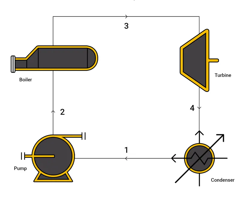
The Rankine cycle is an idealised thermodynamic cycle that turns portion of heat into mechanical work in a constant pressure heat engine. Heat is provided externally to a closed loop in this cycle, which typically uses water (in both liquid and vapour phase) as the working fluid.

• Isentropic Expansion (1-2) - In the turbine, the vapour expands, producing work that can be turned to electricity. As the process advances farther into the two-phase zone, the expansion is restricted by the temperature of the cooling medium and the erosion of the turbine blades caused by liquid entrainment in the vapour stream. To extend the life of turbine blades, exit vapour quality should be more than 90%.

• Isobaric Heat Rejection (2-3) - The vapor-liquid mixture that exits the turbine (2) is condensed at a low pressure, commonly in a surface condenser that uses cooling water. The pressure of the vapour is much below atmospheric pressure in well-designed and maintained condensers, reaching the saturation pressure of the operating fluid at the cooling water temperature.

• Isentropic Compression (3-4) - In the feed pump, the condensate pressure is increased. Pump effort is generally minor due to the low specific volume of liquids and is frequently overlooked in thermodynamic calculations.
• Isobaric Heat Transfer (4-1) - The feed pump sends high-pressure liquid into the boiler, which is heated to saturation temperature. As more energy is added, the liquid evaporates until it is completely transformed to saturated steam (1).

CODE -

clear all 
close all 
clc

%displaying Rankine cycle simulator 

%turbine inlet temperature = Tt
Tt =400;
%turbine inlet pressure = Tp
Tp = 30;
%turbin condensor inlet pressure = Cp
Cp =0.05;
%specific enthalpy
H1 = XSteam('h_pT',30,400)
%Specific Entropy
S1= XSteam('s_ph',30,H1)

T1 = Tt;

%displaying Rankine cycle simulator 
a=fopen('Rankine_cyc','wt');
fprintf(a,'RANKINE CYCLE SIMULATOR \n 1-2 is the isentropic expansion process \n 2-3 is the constant pressure heat rejection process \n 3-4 is the isentropic compression process \n 4-1 is the constant pressure heat addition process');
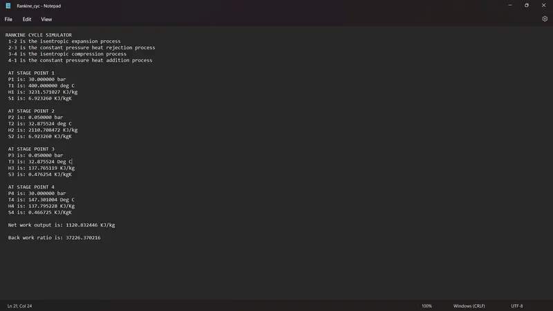
fprintf(a,'\n\n AT STAGE POINT 1')
fprintf(a,'\n P1 is: %f bar',Tp)
fprintf(a,'\n T1 is: %f deg C',T1')
fprintf(a,'\n H1 is: %f KJ/kg',H1')
fprintf(a,'\n S1 is: %f KJ/kgK',S1')

%Isentropic expansion SO S1= S2
S2 = S1
Sf = XSteam('sL_p',0.05);
Sg = XSteam('sV_p',0.05);
Sfg = Sg-Sf
%dryness fraction S1= sf + (x.*Sfg)
X = (S1-Sf)/Sfg
Hf = XSteam('hL_p',0.05);
Hg = XSteam('hV_p',0.05);
Hfg = Hg-Hf;

H2 = Hf + (X.*Hfg);

T2 = XSteam('T_hs',H2,S2);

fprintf(a,'\n\n AT STAGE POINT 2')
fprintf(a,'\n P2 is: %f bar',Cp)
fprintf(a,'\n T2 is: %f deg C',T2')
fprintf(a,'\n H2 is: %f KJ/kg',H2')
fprintf(a,'\n S2 is: %f KJ/kgK',S2')

H3 = Hf;

T3 = T2;

%H4 3-4 is pump work wd = h4-h3 =V3*(p4-p3)
%P4 is Tt and P3 is Cp
V3 = XSteam('vL_p',0.05);

S3 = Sf

fprintf(a,'\n\n AT STAGE POINT 3')
fprintf(a,'\n P3 is: %f bar',Cp)
fprintf(a,'\n T3 is: %f Deg C',T3')
fprintf(a,'\n H3 is: %f KJ/kg',H3')
fprintf(a,'\n S3 is: %f KJ/kgK',S3')

H4 = H3+(V3.*(Tp-Cp));

Sg = XSteam('sV_p',0.05);

Sfg = Sg-Sf

%dryness fraction S1= sf + (x.*Sfg)
X = (S1-Sf)/Sfg

S4 = XSteam('s_ph',Tp,H4);
term = exp(((XSteam('SL_P',30))-S4)/(XSteam('CpL_p',30)))
T4 = (XSteam('Tsat_p',30))/term

%T4 = XSteam('T_hs',H4,S4);

fprintf(a,'\n\n AT STAGE POINT 4')
fprintf(a,'\n P4 is: %f bar',Tp)
fprintf(a,'\n T4 is: %f Deg C',T4')
fprintf(a,'\n H4 is: %f KJ/Kg',H4')
fprintf(a,'\n S4 is: %f KJ/KgK',S4')

T5 = XSteam('Tsat_p',30);
T6 = T5;

S5 = XSteam('sL_p',30);
S6 = XSteam('sV_p',30);

%pump work input = Wp

Wp = V3*(Tp-Cp)

%turbine work output =Wt

Wt =H1-H2;

%Net work output 

Net_wout = Wt-Wp
fprintf(a,'\n\n Net work output is: %f KJ/kg',Net_wout')

%Calculatiing back work ratio = work_turbine/work pump

back_wr = Wt/Wp
fprintf(a,'\n\n Back work ratio is: %f ',back_wr')

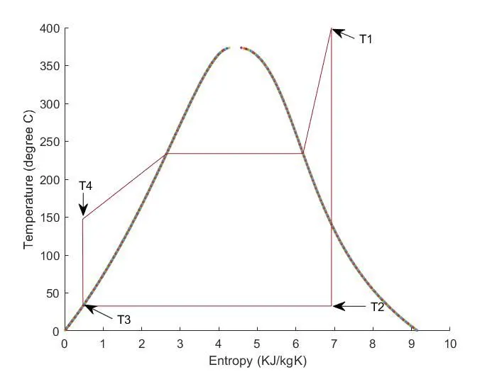
%Plotting T & S diagram

t_range = linspace(0,374.15,500);
figure(1)
hold on
for i= 1:length(t_range)
plot(XSteam('sL_t',t_range(i)),t_range(i),'.')
plot(XSteam('sV_t',t_range(i)),t_range(i),'.')
end

figure(1)
hold on
plot ([S1,S2,S3,S4,S5,S6,S1],[T1,T2,T3,T4,T5,T6,T1])
xlabel 'Entropy (KJ/kgK)' 
ylabel 'Temperature (degree C)'

%Plotting H & S diagram

figure(2)
hold on
for i= 1:length(t_range)
plot(XSteam('sL_t',t_range(i)),XSteam('hL_t',t_range(i)),'.')
plot(XSteam('sV_t',t_range(i)),XSteam('hV_t',t_range(i)),'.')
end

figure(2)
hold on
plot ([S1,S2,S3,S4,S1],[H1,H2,H3,H4,H1])
xlabel 'Entropy (KJ/kgK)' 
ylabel 'Enthalpy (KJ/kg)'

RESULTS

T_S DIAGRAM OUTPUT

H-S DIAGRAM OUTPUT

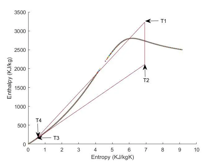
As a result both T-S and H-S diagrams are generated, also the Net work output and back work ratio is calculated.

Step-Wise Explanation

• Initially the inputs are collected as given.
• Started with finding all the State point variables at stage-1 using the XSteam file.
• Then after moving to Stage- 2, the dryness fraction is calculated to further evaluate other state point variables.
• Then similarly for Stage-3 and stage 4 variables the equations are evaluated and the state point variables are found.
• Two of the variables i.e T and S are calculated on 2 more stages to generate the more precise graph and results.
• After that Net work out put is calculated.
• Also the Back work ratio is calculated.
• And finally the graph for T-S diagram and H-S diagram has been plotted by taking all the values evaluated above.
• In both the graphs the Water-Vapour dome is displayed by using values from XSteam at 500 sequencial point, this has made the representation of graphs more meaningfull.

Errors generated during code.

there are lot of errors been generated related to picking up wrong values from XSteam file.

Also there are much of typo errors.

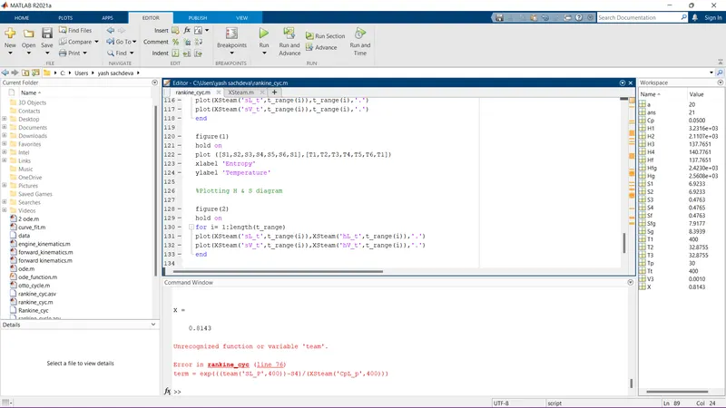
Also considered the temperature instead of pressure in the expression and found wrong values number of times.