Week 4.1 - Genetic Algorithm

The aim of this project is to write a code to optimize the stalagmite function and find the global maxima of the function and thus while doing this program we will be able to understand the concept of Optimization and Genetic Algorithm.

Optimization

Optimization is a decision making process, it helps to find the best results under a set of prioritized criteria or constraints. (or) in general the process of finding maxima or minima of a function under a set of conditions.

In the simplest case, an optimization problem consists of maximizing or minimizing a real function by systematically choosing input values from within an allowed set and computing the value of the function. The generalization of optimization theory and techniques to other formulations constitutes a large area of applied mathematics. More generally, optimization includes finding "best available" values of some objective function given a defined domain (or input), including a variety of different types of objective functions and different types of domains.

Techniques available to perform genetic algorithm

• Deterministic method- In this technique, the output of the model is fully determined by the parameter values and initial conditions and they use specific rules for moving one solution to other.
• Stochastic method-This model possess some inherent randomness, it is a probabilistic approach.

Steps usually involved in an optimal design

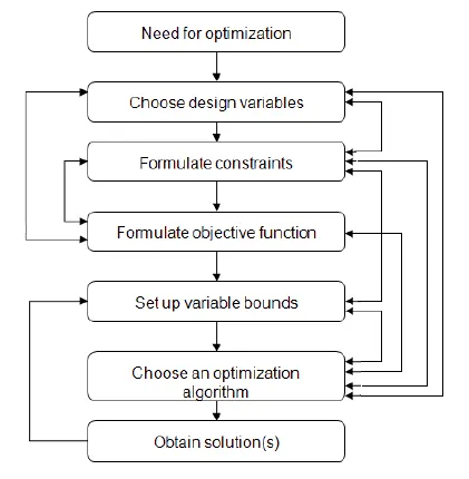
• Variables are the parameters which you have to vary during the optimization process.
• During the optimization process your output should not go beyond the certain limits, those are known as constraints.
• Objective function is as simple as a mathematical forumulae, which can be a predicted mathematical model that includes all the variables as input.
• Variable bounds are the range of the input variable, that will be varied for every iteration to provide an optimized result.
• We need to choose an optimization algorithm to perform the optimization process.

Genetic algorithm

Genetic algorithm is based up on theory of natural evolution that was proposed by Charles Darwin. This algorithm reflects the process of natural selection where the fittest individuals are selected for reproduction in order to produce offspring of the next generation.

The genetic algorithm is a method for solving both constrained and unconstrained optimization problems that is based on natural selection, the process that drives biological evolution. The genetic algorithm repeatedly modifies a population of individual solutions.

Genetic algorithm is one of the optimization process and Matlab provides inbuilt functions for doing genetic algorithm. You can apply the genetic algorithm to solve a variety of optimization problems that are not well suited for standard optimization algorithms, including problems in which the objective function is discontinuous, non-differentiable, stochastic, or highly nonlinear. The genetic algorithm can address problems of mixed integer programming, where some components are restricted to be integer-valued.

The process of natural selection starts with the selection of fittest individuals from a population. They produce offspring which inherit the characteristics of the parents and will be added to the next generation. If parents have better fitness, their offspring will be better than parents and have a better chance at surviving. This process keeps on iterating and at the end, a generation with the fittest individuals will be found.

Five phases are considered in a genetic algorithm.

1. Initialize
2. Fitness function
3. Selection
4. Crossover
5. Mutation

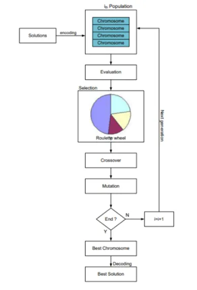
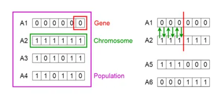
1) Initialization-The process begins with a set of individuals which is called a Population. Each individual is a solution to the problem you want to solve. An individual is characterized by a set of parameters (variables) known as Genes. Genes are joined into a string to form a Chromosome (solution).

In a genetic algorithm, the set of genes of an individual is represented using a string, in terms of an alphabet. Usually, binary values are used (string of 1s and 0s). We say that we encode the genes in a chromosome.

In the initialization we have to decide the population size, higher the population size, will get more combinations, hence we get more accurate results.

2) fitness function- The fitness function determines how fit an individual is (the ability of an individual to compete with other individuals). It gives a fitness score to each individual. The probability that an individual will be selected for reproduction is based on its fitness score.

3) Selection-The idea of selection phase is to select the fittest individuals and let them pass their genes to the next generation. Two pairs of individuals (parents) are selected based on their fitness scores. Individuals with high fitness have more chance to be selected for reproduction.

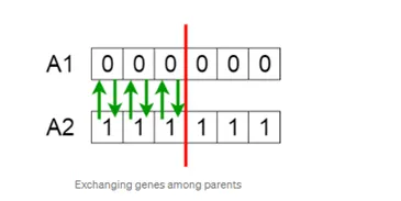
4) Crossover is the most significant phase in a genetic algorithm. For each pair of parents to be mated, a crossover point is chosen at random from within the genes.

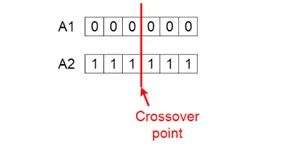
Offspring are created by exchanging the genes of parents among themselves until the crossover point is reached.

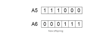
The new offspring are added to the population.

5) Mutation-In certain new offspring formed, some of their genes can be subjected to a mutation with a low random probability. This implies that some of the bits in the bit string can be flipped. Mutation occurs to maintain diversity within the population and prevent premature convergence.

If mutation is not performed, the chromosomes will become too similar to each other, convergence take place soon and results in local minima.

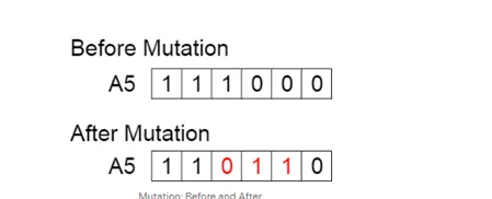
Termination-The algorithm terminates if the population has converged (does not produce offspring which are significantly different from the previous generation). Then it is said that the genetic algorithm has provided a set of solutions to our problem.

The population has a fixed size. As new generations are formed, individuals with least fitness die, providing space for new offspring.

The sequence of phases is repeated to produce individuals in each new generation which are better than the previous generation.

Below is the basic syntax of a genetic algorithm coding.

START
Generate the initial population
Compute fitness
REPEAT
Selection
Crossover
Mutation
Compute fitness
UNTIL population has converged
STOP

Stalagmite function is a mathematical model that helps us to generate local minima’s and maxima’s.

x = ga(fun,nvars,A,b,Aeq,beq,lb,ub) defines a set of lower and upper bounds on the design variables, x, so that a solution is found in the range lb ≤ x ≤ ub. (Set Aeq=[] and beq=[] if no linear equalities exist.)

Below explanation for each of the variables

Aeq Aeq matrix for linear equality constraints

Beq beq vector for linear equality constraints

lb Lower bound on x

ub Upper bound on x

nonlcon Nonlinear constraint function

rngstate optional field to reset the state of the random number generator

solver ga

options options created using optimoptions or exported from the optimization app

• From the below equation we can create the coding for stagalmite function.

`f(x,y)=f_(1,x) f_(2,x) f_(1,y) f_(2,y)`

`f_(1,x)=[sin(5.1πx+0.5)] .^6`

`f_(1,y)=[sin(5.1πy+0.5)] .^6`

`f_(2,x)=exp[-4ln(2) ((x-0.0667) .^2)/0.64]`

`f_(2,y)=exp[-4ln(2) ((y-0.0667) .^2)/0.64]`

1) The code written below will help us to optimize the stalagmite function and to find out the global maxima of the function.

% stalagmite HW to find global Maxima
clear all
close all
clc
% defining our search space
x=linspace(0,0.6,150);
y=linspace(0,0.6,150);
% Initiating the limits
num_cases=50;
% calling the function with 2D Mesh
f=get_stalagmite_max(x,y);

% study-1 statistical behaviour
tic
for i=1:num_cases
    [inputs,fopt(i)]=ga(@stalagmite_max_func,2);
    xopt(i)=inputs(1);
    yopt(i)=inputs(2);
end
study1_time=toc
figure(1);
% creating subplots in the same figure window
subplot(2,1,1);
hold on
surfc(x,y,-f);
shading interp
plot3 (xopt,yopt,-fopt,'Marker','o','MarkerSize',5,'MarkerFaceColor','r');
xlabel('X value');
ylabel('Y value');
title("unbounded inputs")

% optimimum value that the function is predicting for the iteration
subplot(2,1,2);
plot(-fopt);
xlabel('Iterations');
ylabel('Function Maximum');

% study-2 satistical behaviour with upper and lower bounds
tic
for i=1:num_cases
    [inputs,fopt(i)]=ga(@stalagmite_max_func,2,[],[],[],[],[0;0],[1;1]);
    xopt(i)=inputs(1);
    yopt(i)=inputs(2);
end
study2_time=toc
figure(2)
subplot(2,1,1);
hold on
surfc(x,y,-f);
shading interp
plot3(xopt,yopt,-fopt,'Marker','o','MarkerSize',5,'MarkerFaceColor','r');
title('Bounded inputs');
xlabel('X value');
ylabel('Y value');
subplot(2,1,2);
plot(-fopt);
xlabel('Iterations');
ylabel('Function Maximum');

% study-3 increasing GA Iterations
tic
options=optimoptions('ga');
options=optimoptions(options,'populationsize',300);
tic
for i=1:num_cases
    [inputs,fopt(i)]=ga(@stalagmite_max_func,2,[],[],[],[],[0;0],[1;1],[],[],options);
    xopt(i)=inputs(1);
    yopt(i)=inputs(2);
end
study3_time=toc
figure(3)
subplot(2,1,1)
hold on
surfc(x,y,-f)
shading interp
plot3(xopt,yopt,-fopt,'Marker','o','MarkerSize',5,'MarkerFaceColor','r');
title('Bounded inputs with increased population size');
xlabel('X value');
ylabel('Y value');
subplot(2,1,2)
plot(-fopt)
xlabel('Iterations');
ylabel('Function Maximum');
tic

2) Coding for stalagmite_max_func function to slove the stalagmite equation

% stalagmite function for running the program
function [f]=stalagmite_max_func(input_vector)
x=input_vector(1);
y=input_vector(2);
f1X=(sin(5.1*pi*x+0.5))^6;
f1Y=(sin(5.1*pi*y+0.5))^6;
f2X=exp(-4*log(2)*((x-0.0667)^2/0.64));
f2Y=exp(-4*log(2)*((y-0.0667)^2)/(0.64));
f=-(f1X*f1Y*f2X*f2Y);
end

3) Coding for get_stalagmite_max function for creating the meshgrid and initilazie the inputs

% stalagmite function for creating 2D mesh in global max
function [f]=get_stalagmite_max(x,y)
x=linspace(0,0.6,150);
y=linspace(0,0.6,150);
[xx,yy]=meshgrid(x,y);
for i=1:length(xx)
    for j=1:length(yy)
        input_vector(1)=xx(i,j);
        input_vector(2)=yy(i,j);
        f(i,j)=stalagmite_max_func(input_vector);
    end
end
end

• Maxima and minima of the function can be plot by using the same code by just applying the negative and positive sign to the formulae.
• ‘num_cases ‘ command will give the stalagmite function the number of iteration.
• Evaluation of study time can be displayed by using ‘tic’ and ‘toc’ command.
• ‘surfc’ command is used for plotting the 3D plots or giving a surface finish to the plot.
• 'subplot' command is used for creating a subplot in the same figure window.
• While using surfc applying the -ve sign to the function will generate the surface upside down which will be quite good to get the maxima of the function, as it will provide positive value for the maxima using the -ve sign.
• In study-3 ‘optimoptions’ command is used to increase the size of population. It will work on the large set number which will be led to increase the possibilities of finding the better fitness of the function but the time for evaluation will increase.

1) The plot for the first case study-1 statistical behaviour of the GA.

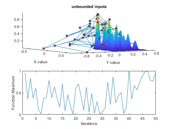
From the above plot we can conclude that the GA try to find the best mutation within the small group of population within a short time period but the final result is not accurate as expected.

2) Second plot will give us details of case study-2 statistical behaviour of the GA with upper and lower bounds.

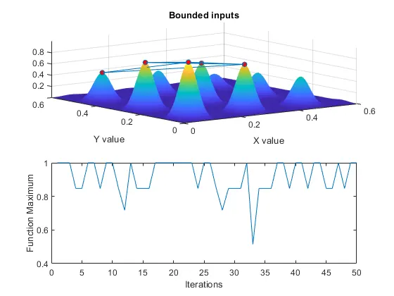
The difference over here is in providing the upper and the lower limit in the ga so that the search space is reduced with the upper and lower boundary.

3) Plot-3 with increased the GA iterations in case study-3.

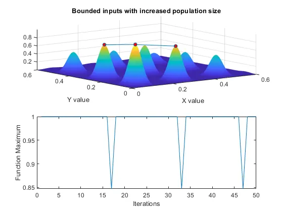
This plot will gives us an accurate result while comparing to the other two plots. But while increasing the iterations (population size) the simulation time will increase with an acceptable output.

4) Plot-4 Here we are increasing the GA Iterations (population size) in study-3 GA for getting a more accurate plot and te acceptable results.

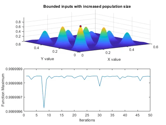
Here we will get the more accurate global maxima by the ga function by crossing the best fit chromosome and give us the best offspring from the given iterations.By increasing the initial population size of the ga we will get the best results and ga is useful for optimizing the function.

Thus we can conclude that In the initialization we have to decide the population size, higher the population size, will get more combinations, hence we get more accurate results.