Project 2 - Rankine cycle Simulator
Aim of the project
The aim of the project is to understand the process of Rankine cycle and to create a Matlab program which calculate the state points variables of the Rankine cycle based on user inputs by using the standard Xsteam library to get the steam table data for water and create the corresponding plots T-S (Temperature-entropy) and H-S (Enthalpy-entropy) for the given set of inputs with proper labelling and detailing.
The first step of this project is to understand the concept of Thermodynamic cycle and the working of a Rankine cycle then find out the equations and list out the state point variables.
Thermodynamic cycle
A thermodynamic cycle consists of a linked sequence of thermodynamic processes that involve transfer of heat and work into and out of the system, while varying pressure, temperature, and other state variables within the system, and that eventually returns the system to its initial state.
Theory of Rankine cycle
The Rankine cycle is an idealized thermodynamic cycle of a constant pressure heat engine that converts part of heat into mechanical work. In this cycle, the heat is supplied externally to a closed loop, which usually uses water (in a liquid and vapor phase) as the working fluid.
Heat energy is supplied to the system via a boiler where the working fluid(typically water) is converted to a high pressure gaseous state (steam) in order to turn a turbine. After passing over the turbine the fluid is allowed to condense back into a liquid state as waste heat energy is rejected before being returned to boiler, completing the cycle.
The Rankine cycle is the fundamental operating cycle of all power plants where an operating fluid is continuously evaporated and condensed. The selection of operating fluid depends mainly on the available temperature range.
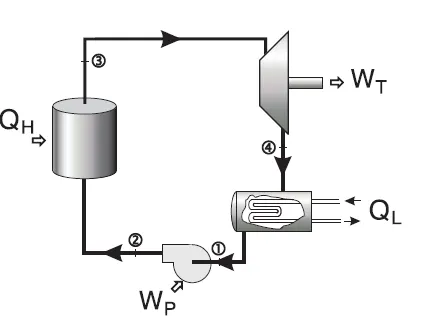
State points of Rankine cycle
1) Isentropic compression (compression in centrifugal pumps) – The liquid condensate is compressed adiabatically from state 1 to state 2 by centrifugal pumps (usually by condensate pumps and then by feed water pumps). The liquid condensate is pumped from the condenser into the higher pressure boiler. In this process, the surroundings work on the fluid, increasing its enthalpy (h = u+pv) and compressing it (increasing its pressure). On the other hand, the entropy remains unchanged. The work required for the compressor is given by WPump = H2 – H1.
2) Isobaric heat addition (in a heat exchanger – boiler) – In this phase (between state 2 and state 3), there is a constant-pressure heat transfer to the liquid condensate from an external source since the chamber is open to flow in and out. The feed water (secondary circuit) is heated to the boiling point (2 → 3a) of that fluid and then evaporated in the boiler (3a → 3). The net heat added is given by Qadd = H3 – H2.
3) Isentropic expansion (expansion in a steam turbine) – Steam from the boiler expands adiabatically from state 3 to state 4 in a steam turbine to produce work and then is discharged to the condenser (partially condensed). The steam works on the surroundings (blades of the turbine) and loses an amount of enthalpy equal to the work that leaves the system. The work done by the turbine is given by WT = H4 – H3. Again the entropy remains unchanged.
4) Isobaric heat rejection (in a heat exchanger) – In this phase, the cycle completes by a constant-pressure process in which heat is rejected from the partially condensed steam. There is heat transfer from the vapor to cooling water flowing in a cooling circuit. The vapor condenses, and the temperature of the cooling water increases. The net heat rejected is given by Qre = H4 – H1.
In general, the thermal efficiency nth, of any heat engine is defined as the ratio of the work it does, W, to the heat input at the high temperature, QH.
nth=W/QH
The work done by the pump to compress water (Wpump) can be represented as the change in enthalpy (H) of the water (fluid) before entering the pump and after leaving the pump:
Wpump=H2−H1
Qin=H3−H2
Wturbine=H3−H4
Qout=H4−H1
The energy balance for the whole cycle is then can be expressed via the following equation:
(Qin−Qout)−(Wturbine−Wpump)=0(Qin−Qout)−(Wturbine−Wpump)=0
The net work done by the system is Wturbine-Wpump. Therefore, the thermal efficiency of this cycle can be presented as follows:
η=WnetQin=1−QoutQin
Net work output of the cycle
The net work output of the cycle equals the difference between the turbine work output and the pump work input.
wnet,out = wturb,out - wpump,in
Back work ratio
The compressor requires to work for its operation whereas turbine produces work after operation. Due to this, the compressor work is said to be negative and turbine work is considered positive. we can define back work ratio as the ratio between the work done by the compressor to the work done by turbine in the thermal power plant. The compressor work is derived from the turbine itself, that is around thirty percent of the turbine work is translated to compressor work.
The turbine work is represented by h2-h1 and compressor work is represented by h4-h3. The total work done is represented by h1-h4.
Back work ratio = Compressor work/Turbine work = (h4-h3)/(h2-h1)
Matlab code for Rankline cycle simulator
% Project-2 Rankie cycle
clear all
close all
clc
% Giving the header to the simulator
fprintf('RANKINE CYCLE SIMULATOR');
fprintf('\n \n State Points');
% State points of Rankine cycle
fprintf('\n 1-2 is Isentropic expansion in the turbine');
fprintf('\n 2-3 is constant pressure heat rejection by condenser');
fprintf('\n 3-4 is Isentropic compression in the pump');
fprintf('\n 4-1 is constant pressure heat addition by the boiler');

% Entering the given Inputs
P1=input('\n \nEnter the pressure at the Turbine inlet (in bar):');
T1=input('Enter the temperature at the Turbine inlet (in degree celsius):');
P2=input('Enter the pressure at the Condenser (in bar):');

% initiating the variables for state point-1
P1;
T1;
% calling the corresponding values of h and s from Xsteam
H1=XSteam('h_pt',P1,T1);
S1=XSteam('s_pt',P1,T1);
% To get the points in between the state variables
ts1=XSteam('Tsat_p',P1);
sg1=XSteam('sV_p',P1);
sf1=XSteam('sL_p',P1);
sfg1=sg1-sf1;
hf1=XSteam('hL_p',P1);
hg1=XSteam('hV_P',P1);
hfg1=hg1-hf1;
% Displaying the parameters of state point-1
fprintf('\n RESULTS');
fprintf('\n At state point 1');
fprintf('\n P1 is : %f bar',P1);
fprintf('\n T1 is : %f deg celsius',T1);
fprintf('\n H1 is : %f kj/kg',H1);
fprintf('\n S1 is : %f kj/kgk',S1);

% variables for state point-2
P2;
S2=S1;
% calling the corresponding state point variables from Xsteam
low_cpv=XSteam('CpV_p',P2);
high_cpL=XSteam('CpL_p',P1);
% To get the points in between the state variables
sf2=XSteam('sL_p',P2);
sg2=XSteam('sV_P',P2);
% By applying the thermodynamic equations finding the corresponding values
% x=((S2-sf2)/(sg2-sf2))
sfg2=sg2-sf2;
hf2=XSteam('hL_p',P2);
hg2=XSteam('hV_p',P2);
hfg2=hg2-hf2;
ts2=XSteam('Tsat_p',P2);

%Dryness fraction
if(S2<=sg2)
    X2=(S2-sf2)/(sfg2);
else
    X2=1;
end
 % Calculating T based on the liquid state by thermodynamic equations
if(X2<1)
    T2=ts2;
else
    T2=(ts2+273.15)*exp((S2-sg2)/low_cpv);
    T2=T2-273.15;
end
if(X2<1)
    H2=hf2+X2*hfg2;
else
    H2=hg2+low_cpv*(T2-ts2);
end
v2=XSteam('v_ph',P2,H2);

% Displaying the result of state point-2
fprintf('\n \n At state point 2');
fprintf('\n P2 is : %f bar',P2);
fprintf('\n T2 is : %f deg celsius',T2);
fprintf('\n H2 is : %f kj/kg',H2);
fprintf('\n S2 is : %f kj/kgk',S2);
fprintf('\n X2 is : %f',X2);

% variables for state point-3
T3=ts2;
P3=P2;
S3=sf2;
H3=hf2;
V3=XSteam('vL_p',P3);
% Displaying the result of state point-3
fprintf('\n \n At state point 3');
fprintf('\n P3 is : %f bar',P3);
fprintf('\n T3 is : %f deg celsius',T3);
fprintf('\n H3 is : %f kj/kg',H3);
fprintf('\n S3 is : %f kj/kgk',S3);

% variables for state point-4
P4=P1;
S4=S3;
%V4=V3;
W_pump=V3*(P4-P3)*100;
H4=W_pump+H3;
term=exp((sf1-S4)/high_cpL);
T4=ts1/term;
% Displaying the result of state point-4
fprintf('\n \n At state point 4');
fprintf('\n P4 is : %f bar',P4);
fprintf('\n T4 is : %f deg celsius',T4);
fprintf('\n H4 is : %f kj/kg',H4);
fprintf('\n S4 is : %f kj/kgk',S4);

% Net work output calculation
W_turbine=H1-H2;
Net_Work=(W_turbine-W_pump);
Q_in=H1-H4;
Q_out=H2-H3;

% Thermal efficiency
n_T=Net_Work/Q_in;
n=n_T*100;

% Back work ratio
BWR=W_pump/W_turbine;

% Specific steam consumption
SSC=3600/Net_Work;

% displaying the calculated results
fprintf('\n \n W_turbine is : %f kj/kg',W_turbine);
fprintf('\n W_pump is : %f kj/kg',W_pump);
fprintf('\n W_net is : %f kj/kg',Net_Work);
fprintf('\n N_therm is : %f percent',n);
fprintf('\n S.S.C is : %f kg/kwh \n',SSC);

% To find the variables on saturation lines(liquid & vapour)
temp=linspace(0,400,1000);
for i=1:length(temp)
    H_L(i)=XSteam('hL_T',temp(i));
    H_V(i)=XSteam('hV_T', temp(i));
    S_L(i)=XSteam('sL_T',temp(i));
    S_V(i)=XSteam('sV_T',temp(i));
end

% Plot of T-S
figure(1)
hold on
plot([S_L S_V],[temp temp]);
plot([S1 S2 S3 S4 sf1 sg1 S1], [T1 T2 T3 T4 ts1 ts1 T1]);
text(S1,T1,'1');
text(S2,T2,'2');
text(S3,T3,'3');
text(S4,T4,'4');
text(sf1,ts1,'4a');
text(sg1,ts1,'1a');
title('T-S Diagram of Rankine cycle');
xlabel('Entropy[S] (KJ/KGK)');
ylabel('Temperature[T] (Deg celsius)');
axis([0,10,0,450]);

% Plot of H-S
figure(2)
hold on
plot([S_L S_V],[H_L H_V]);
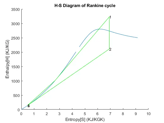
plot([S1 S2 S3 S4 sf1 S1],[H1 H2 H3 H4 hf1 H1], 'Color','g');
text(S1,H1,'1');
text(S2,H2,'2');
text(S3,H3,'3');
text(S4,H4,'4');
title('H-S Diagram of Rankine cycle');
xlabel('Entropy[S] (KJ/KGK)');
ylabel('Enthalpy[H] (KJ/KG)');
axis([0,10,0,3500]);
hold off- First we are writing data (header) to the text file then writing the state points using ‘fprintf’ command.
- The next step is to requesting for user input by using the ‘input’ command.
- Then we are initiating the corresponding state point variables (enthalpy, entropy, etc) values of the user inputs from the ‘Xsteam’ file and simulate it by using ‘fprintf’.
- XSteam provides accurate steam and water properties from 0 - 1000 bar and from 0 - 2000 deg celsius according to the standard IAPWS IF-97.
- XSteam take 2 or 3 arguments. The first argument must always be the steam table function you want to use and the other arguments are the inputs to that function.
- XSteam('h_pt',P1,T1) will written the value of enthalpy(H) of water at Pressure(P1)bar and temperature(T1) deg celsius, ie First the wanted property then the wanted input properties.
- h_pT- Entalpy as a function of pressure and temperature.
- s_ph- Specific entropy as a function of pressure and enthalpy.
- By applying the thermodynamic property and the equations we can find out the required variables. This process is repeated for all state points and simulate the result by using ‘fprintf’ command.
- Finally, the T-S and H-S diagram with saturation lines is generated on the plot.
Output screen
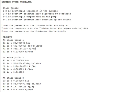
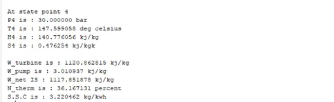
PLOTS
1) T-S diagram
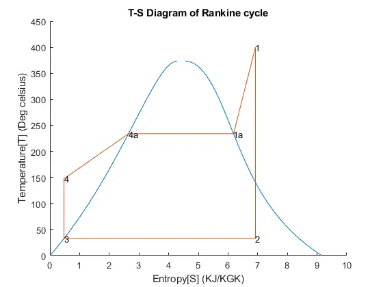
From the above T-S plot,
- Isentropic expansion 1-2 (expansion in a steam turbine)
- Isobaric heat rejection 2-3 (in a heat exchanger)
- Isentropic compression 3-4(compression in centrifugal pumps)
- Isobaric heat addition 4-1 (in a heat exchanger – boiler)
2) H-S diagram
Conclusion
Thus we have understand the working principle of Rankine cycle and successfully simulate the Rankine cycle by using Matlab and created the corresponding plots T-S and H-S for the given set of inputs.
In an ideal Rankine cycle the pump and turbine would be isentropic i.e., the pump and turbine would generate no entropy and hence maximize the net work output. Processes 1–2 and 3–4 would be represented by vertical lines on the T-S diagram and more closely resemble that of the Carnot cycle. The Rankine cycle shown here prevents the state of the working fluid from ending up in the superheated vapor region after the expansion in the turbine, which reduces the energy removed by the condensers.
References
https://www.thermopedia.com/content/1072/
https://in.mathworks.com/help/physmod/simscape/ug/rankine-cycle-steam-turbine.html
https://www.e-education.psu.edu/eme812/node/708
https://drive.google.com/file/d/1RK_fvrOj38CIaQvmLT1S3daqHnxKCGU-/view