Week 4.1 - Genetic Algorithm
GA and Stalagmite
Aim : To write a code in MATLAB to optimize the stalagmite function and find the global maxima of the function.
Objectives :
- To find out Global Maxima of stalagmite function
- Optimization will be done for three cases:
- with unconstrained inputs
- with constrained inputs (Lower and Upper bounds)
- with constrained inputs & increased population size
Theory :
Stalagmite Function :
- A stalagmite is an upward growing mound of mineral deposits on the floor of cave.
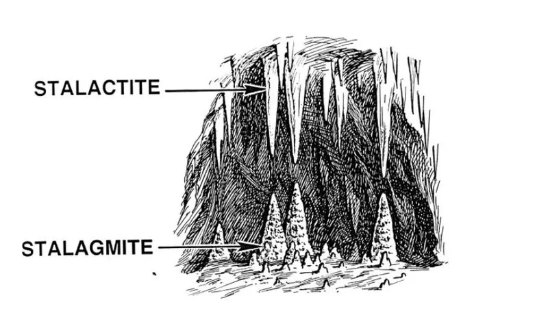
- A stalagmite function generally refers to the function with which we are generating values over a stalagmite kind of surface for finding out the local and global maxima and minima of that particular given function.
- The stalagmite function is a Mathematical model that helps generate local minima and maxima. It is a three-dimensional function and the way the function is designed is that it has a lot of local maxima or minima.
- In MATLAB for this we are using a method called ‘optimization’.
- Optimization is done by systematically choosing input values from within an allowed set and computing the results of the function.
- In MATLAB to perform optimization we use ‘Genetic Algorithm’ method which is a inbuild function in MATLAB to find the global maxima of the given stalagmite function
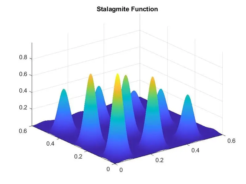
The Stalagmite function is given as,
`f_(1,x)=[sin⋅(5.1πx+0.5)]^6`
`f_(1,y)=[sin⋅(5.1πy+0.5)]^6`
`F_(2,x)=exp[-4 ln(2) (x-0.0667)^2/0.64 ]`
`F_(2,y)=exp[-4 ln(2) (y-0.0667)^2/0.64 ]`
`F(x,y)=f_(1,x)⋅f_(1⋅y)⋅f_(2,x)⋅f_(2,y)`
What is Optimization?
- Optimization is the process of making something better.
- Optimization refers to finding out the values of the inputs in such a way that we get a best output values.
- Optimization is basically area of study that deals with how to minimize and maximize a particular function which depends on multiple input parameters.
- Stochastic optimization refers to a field of optimization algorithms that explicitly use randomness to find the optima of an objective function, or optimize an objective function that itself has randomness
-
Optimization Problems :
Maximize Fuel Efficiency
Minimize Risk
Maximize Profit
Objective Function :
- An Objective function expresses the main aim of the model which is either to be minimized or maximized
- A set of unknowns or variables which control the value of the objective function.
- A set of constraints that allow the unknowns to take on certain values but exclude others.
Genetic Algorithm(GA)
Genetic Algorithm(GA) is search-based optimization technique based on the principle of Genetics and Natural selection. It is frequently used to find optimal or near-optimal solution of difficult problems otherwise it will take a lifetime to solve. It is frequently used to solve optimization problems, in research and in machine learning.
How does the Genetic Algorithm work?
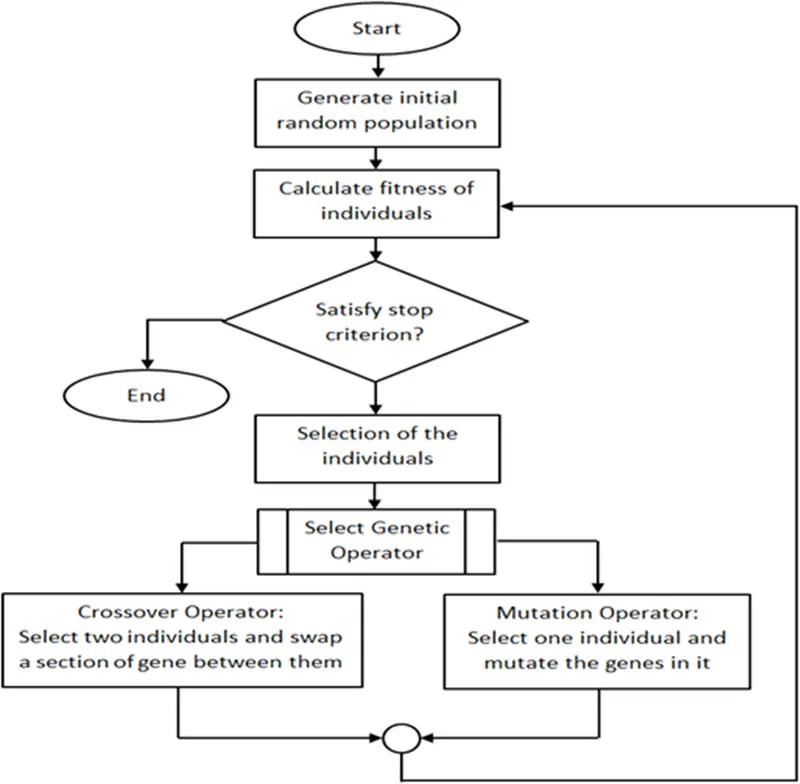
The genetic algorithm works on a population using a set of operators that are applied to the population. A population is a set of points in the design space. The initial population is generated randomly by default. The algorithm computes the next generation of the population using the fitness of the individuals in the current generation.
Flowchart of Genetic Algorithm :
Understanding ga solver (Genetic Algorithm) :
ga uses ‘genetic algorithm’ technique to find out minimum of function.
Syntax for defining ‘ga’(Genetic Algorithm) in MATLAB –
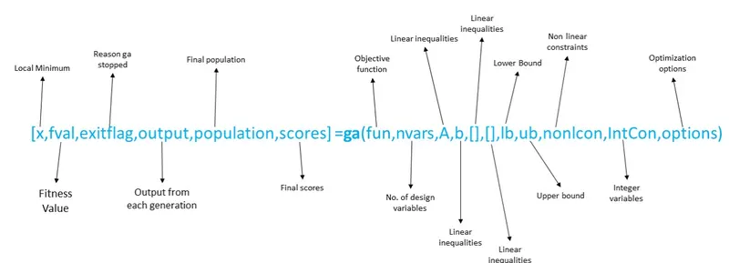
- x= ga(fun,nvars)
where,
x= optimal solution/variables;
fun= objective function;
nvars= Number of Variables;
sometimes [x,fval] is used instead of ‘x’ where ‘fval’ gives objective function value at the solution.
- x= ga(fun,nvar,A,B,Aeq,Beq,lb,ub)
where,
A,B= Linear inequality constraints
Aeq,Beq= Linear equality constraints
If there are no linear equalities and inequalities, then A,B,Aeq,Beq are set to’[ ]’.
- x= ga(fun,nvar,A,B,Aeq,Beq,lb,ub,nonlcon,intCon,options)
where,
nonlcon= Nonlinear Constraints
IntCon= Integer Values
options= Optimization Options
If there are no nonlinear constraints and integer values, the nonlcon and intCon are set to ‘[ ]’.
Tips:
If you run this example without the ‘rng default’ command, your results can differ, because ga is a stochastic algorithm
Stochastic optimization methods are optimization methods that generate and use random variables. For stochastic problems, the random variables appear in the formulation of the optimization problem itself, which involves random objective functions or random constraints. Stochastic optimization methods also include methods with random iterates.
Add Visualization :
- To visualize solver performance while its running, set a ‘PlotFcn’ option using optimoptions.
- In this case, select two plot functions in a cell array.{}
- Set ‘gaplotbestf’, which plots the best and mean score of the population at every generation.
- Also set ‘gaplotstopping’ which plots the percentage of stopping criteria satisfied.
opts=optimoptions(@ga,’PlotFun’,{@gaplotbestf,@gaplotstopping});
Now Run ga solver, including the ‘opts’ argument.
[x,Fval,exitFlag,output]=ga(FitnessFunction,numberOfVariables,[],[],[],[],[],[],[],opts);
Specify Population Options:
Population options can have a large effect on solver performance.
The speed of each iteration depends on the population size: a larger population leads to slower iterations. Conversely, a larger population leads to ga exploring more thoroughly, so can lead to a better solution. Similarly, a wider initial range can lead to more thorough exploration, but can require a larger population to explore the wider range with a similar thoroughness.
MATLAB Programing:
Crate Visualization of Stalagmite Function and function calls:
Crate Visualization of Stalagmite Function and fuction calling:
clear all;
close all;
clc;

x=linspace(0,0.6,150);
y=linspace(0,0.6,150);

[XX YY]=meshgrid(x,y);

for i=1:length(XX)
 for j=1:length(YY)
     input_vector(1)=XX(i,j);
     input_vector(2)=YY(i,j);
     f(i,j)=stalagmite_demo(input_vector);
 end
end

figure(1)
surfc(XX,YY,-f)
shading interp
title('Stalagmite Function')
saveas(figure(1),'stalagmite_function','jpg')
GA with un-constrained inputs:
num_cases= 50;
rng default  % for reproducing same result

FitnessFunction = @stalagmite_demo;
numberOfVariables = 2;
tic;
for k=1: num_cases;
[X,Fval(k)]=ga(FitnessFunction,numberOfVariables);
x_opt(k)=X(1);
y_opt(k)=X(2);
end
Time_1=toc;
display(['Time taken by unbounded ga =' num2str(Time_1),'sec'])
figure(2);
subplot(2,1,1)

surfc(XX,YY,-f)
xlabel('X');
ylabel('Y');
zlabel('f(x,y)')
title('Un-Bounded input Optimization');
shading interp
hold on
plot3(x_opt,y_opt,-Fval,'marker','o','MarkerSize',6,'MarkerFaceColor','r');

subplot(2,1,2)
plot(-Fval,'marker','o','MarkerFacecolor','r')
xlabel('No. of iteration')
ylabel('Max. Function Value')
saveas(figure(2),'GA_With_Unconstrined_inputs','jpg')
Bounded Limit
Bunded Limit
num_cases= 50;
%rng default  % for reproducing same result

FitnessFunction = @stalagmite_demo;
numberOfVariables = 2;
tic;
for k=1: num_cases;
[X,Fval(k)]=ga(FitnessFunction,numberOfVariables,[],[],[],[],[0;0],[1;1]);
x_opt(k)=X(1);
y_opt(k)=X(2);
end
Time_2=toc;
display(['Time taken by bunded ga=',num2str(Time_2),'sec'])
figure(3);
subplot(2,1,1)

surfc(XX,YY,-f)
xlabel('X');
ylabel('Y');
zlabel('f(x,y)')
title('Bounded input Optimization');
shading interp
hold on
plot3(x_opt,y_opt,-Fval,'marker','o','MarkerSize',6,'MarkerFaceColor','r');

subplot(2,1,2)
plot(-Fval,'marker','o','MarkerFaceColor','r')
xlabel('No. of iteration')
ylabel('Max. Function Value')
saveas(figure(3),'GA_Bounded_input_optimization','jpg')
Bounded inputs and increased population
num_cases= 50;
rng default  % for reproducing same result

FitnessFunction = @stalagmite_demo;
numberOfVariables = 2;
opts.PopulationSize=500;
tic;
for k=1: num_cases;
[X,Fval(k)]=ga(FitnessFunction,numberOfVariables,[],[],[],[],[0;0],[0.6;0.6],[],[],opts);
x_opt(k)=X(1);
y_opt(k)=X(2);
end
Time_3=toc;
display(['Time taken by bounded limt and increased population size of ga= ',num2str(Time_3),'sec'])
figure(4);
subplot(2,1,1)
surfc(XX,YY,-f)
xlabel('X');
ylabel('Y');
zlabel('f(x,y)')
title('Bounded Inputs and Increase population Size');
shading interp
hold on
plot3(x_opt,y_opt,-Fval,'marker','o','MarkerSize',6,'MarkerFaceColor','r');
subplot(2,1,2)
plot(-Fval,'marker','o','MarkerFaceColor','r')
%ytickformat('%.6f')
xlabel('No. of iteration')
ylabel('Max. Function Value')
saveas(figure(4),'GA_Bounded_incerease_population','jpg')
Explation:
1. First learn to Create a function of stalagmite.After that in the main programing file call the stalgmite function. We use stalgmite function in double for loop so we can insert each x,y value in stalgmite function to generate z value. To visualize the stalagmite we use surfc command.
2. Now move towards the actual program of optimization using GA. In the first case we use GA with un-constrained inputs for it we use simple syntax that includes fitness function and number of variables. We have to run 'ga' 50 times so we use for loop with case value is 50. In each type we calculate time taken by 'ga' using tic and toc command. By using subplot we will get visual that we run 50 iteration of 'ga' and we get 50 different values and which are lies between 0 to 1.
3. For better solution we have to define search space to 'ga' by giving upper and lower bound. and all other processes same as above statement.
4. Now we can observed that we are lying towards the optimum solution. But in addition we can increase the population size so we will get exact maximum solution having max value 1. It increase time for 'ga'
Results :
Study 1- Statistical Behaviour
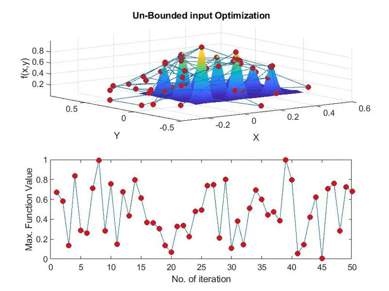
In the above plot, it can be observed that how random number of inputs selected by ga to create optimum solution. Large number of red dots which shows how optimum values falls around stalagmite function. In first case ‘ga’ select random numbers of sampling to create maximum point.
Study 2- Statistical Behaviour with Upper and Lower bounds.
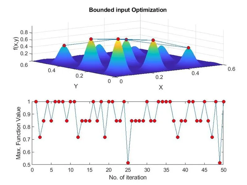
The above result show the convergence of x and y values. The number of red dots are less compared to pervious plot. Here we are try to approach the optimum solution by giving bound to ‘ga’.
Study 3- Statistical Behaviour with increasing iterations of GA
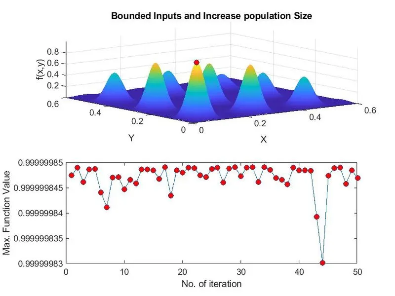
In this study, the number of iterations is increased to 500 to converge the solution at best point to find the global maxima of the function. Howerever incereased in population size , also incereases time to run ga. we can see that we got to many solutions having value 1.
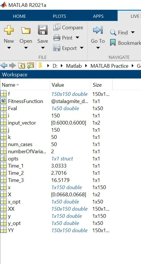
Workspace Values :
Error:
No major error observed during the coding
References :