Project 2 - Rankine cycle Simulator
Simulation of Rankine Cycle using MATLAB :
Aim: To Simulate the Rankine Cycle and plot the corresponding T-S and H-S plot using MATLAB.
Objective:
- Calculate the state points of the Rankine Cycle based on the given inputs.
- Plot the corresponding T-S and H-S plot for the given inputs
- Calculate Net work output and Back work ratio.
Note: The standard XSteam library is used to get the steam table data for water, which is used to calculate the points between the state variables.
Introduction:
- Rankine Cycle is an idealized thermodynamic cycle describing steam turbines or reciprocating steam engines. In this area, fluid flows between a heat source and heat sink.
- Heat energy is supplied to the system via a boiler where water is converted into a high-pressure steam and injected on a turbine in order to rotate.
- After passing over the turbine the fluid is condensed by rejecting heat and converted into the water in condenser.
- Again water is pumped into the storage of boiler and Rankine cycle is completed
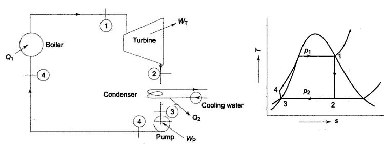
Fig. Basic Outlet diagram for Steam Turbine follows Rankine Cycle
- Process 1-2 : The dry saturated high pressure vapour expands through a turbine and rotate turbine for generating power. This decreases temperature ans pressure of the vapour. Process 1-2 isisentropic expansion.
- Process 2-3 : The wet vapour then enters a condenser, where it is condense at a constant pressure to become a saturated liquid. Process 2-3 is constant pressure heat rejection in condenser
- Process 3-4 : The Working fluid is pumped from low to high pressure. Process 3-4 is isentropic compression.
- Process 4-1 : The high pressure liquid enters a boiler, where it is heated at constant pressure by an external heat source to become a dry saturated vapour. Process 4-1 is constant pressure heat addition in boiler.
-Again above Cycle continues to generate electricity from steam turbine.
Thermal Efficiency of Rankine Cycle:
The work performed by the turbine, which is decreased by the pump divided by the heat energy received by the boiler is known as the Rankine cycle thermal efficiency.
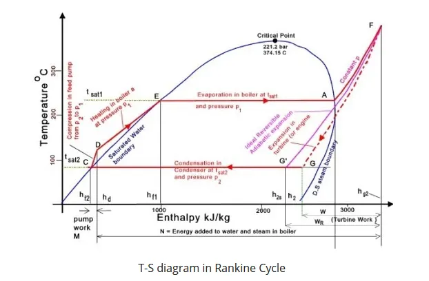
The water vapor absorbs a calorific value that can calculate by the below-given equation:
Qin= m(hF – hD)
The boiler converts the water into superheated steam. This steam is delivered to the turbine. Then, as the line F-G in the above figure shows, the water vapor thermal energy converts into kinetic energy. The decrease in enthalpy uses to compute the amount of kinetic energy produced by a steam turbine. It can calculate by using the below-given equation:
Wout= m(hF-hG)
The boiler converts the water into superheated steam. This steam is delivered to the turbine. Then, as the line F-G in the above figure shows, the water vapor thermal energy converts into kinetic energy. The decrease in enthalpy uses to compute the amount of kinetic energy produced by a steam turbine. It can calculate by using the below-given equation:
Qout= m(hG-hC)
After the condensation process, the condensed water is pumped again into the boiler by increasing the water pressure. As shown in the above diagram (line C to D), the enthalpy of the water has not increased much. It means that the energy released into the air is less important. You can calculate the input energy value using the below-given formula
Win= m(hD-hC)
Now finally, the Rankine cycle efficiency can be calculated by the following formula:
Thermal Efficiency = [(Work Output — Work input)/Heat entered into the system]
- The overall thermal efficiency of the latest nuclear power plant having a Rankine cycle is about 33%. So, 3000 MWth of fission reaction heat is required to make 1000 MWe of electricity.
- Supercritical fossil fuel power plant operating at supercritical pressures (such as higher than 22.1 MPa) has an efficiency of up to 43 percent.
- Subcritical fossil fuel power plants operating at critical pressures (less than 22.1 MPa) may accomplish efficiency between 36% to 40%.
How to increase the efficiency of the Rankine Cycle?
The efficiency of the Rankine cycle can be improved in following way:
- Reduce the average temperature
- Superheat the steam
- Increase boiler pressure
- Decrease the condenser pressure
Program :
clear all
close all
clc


disp('<strong>General Outlet of Steam Turbine</strong>')
figure(1)
imshow('working.jpg')
title('Basic outlet diagram of Steam Turbine ','bold','FontSize',14)
disp('----------------<strong>Rankine Cycle Simulator</strong>----------------');
disp('1-2 : Isentropic Expansion in the Turbine');
disp('2-3 : Constant Pressure Heat rejection by the Condensor');
disp('3-4 : Isentropic Compression in the Pump')
disp('4-1 : Constant Pressure Heat addition by the boiler')

p1= input('Enter the Pressure at the Turbine Inlet(in bar) : ')
t1= input('Enter the Temperature at the Turbine Inlet(in deg.c) : ')
p2= input('Enter the Pressure at the condensor(in bar) : ')

% p1=30;
% t1=400;
% p2=0.05;
% Condition at the inlet of Turbine
tsat=XSteam('Tsat_p',p1);
if t1>tsat
    tsup=t1;
    h1= XSteam('h_pT',p1,tsup);
    s1= XSteam('s_pT',p1,tsup);
elseif t1==tsat
    h1= XSteam('hL_p',p1);
    s1= XSteam('sL_p',p1);
else
    disp('Temperature entered must be greater than or equal to saturation temperature')
end

sf1=XSteam('sL_p',p1);                      % saturated liquid entropy
sg1=XSteam('sV_p',p1);                      % saturated vapour entropy

% Condition at the Condenser inlet or the Turbine exhaust
t2= XSteam('Tsat_p',p2);
hf2= XSteam('hL_p',p2);
hg2= XSteam('hV_p',p2);
s2=s1;                                      % Isentropic Expansion
sg2= XSteam('sV_p',p2);                     % saturated vapour entropy
sf2= XSteam('sL_p',p2);                     % saturated liquid entropy
x2= (s2-sf2)/(sg2-sf2);                     % Dryness Fraction

h2= hf2 + (x2*(hg2-hf2));


% Condition at the Condenser exit
p3=p2;
t3=t2;
h3=hf2;
s3=sf2;

% Condition at boiler inlet
p4=p1;                          % addition of heat at constant pressure
s4=s3;
cp4= XSteam('Cp_ps',p4,s4);
cv4= XSteam('Cv_ps',p4,s4);

gamma= cp4/cv4;
t4= t3*(p4/p3)^(1-(1/gamma));   % Finding the temp. at outlet of pump

vf= XSteam('vL_p',p3);          % Finding Volume at inlet pressure of pump 'p3'
Wp= vf*(p1-p2)*100;             % In KJ multiply 100 % p4=p1 and p3=p2
h4= Wp+h3;

Wt= h1-h2;                      % Work Output from Turbine
Qin = h1-h4;                    % Heat input
Qout= h2-h3 ;                   % Heat rejected
Wnet= Wt-Wp;                    % Net work

Thermal_eff= (Wnet/Qin)*100 ;   % thermal efficiency
ssc= 3600/Wnet;                 % Specific Fuel Consumption
bwr= Wp/Wt;                     % Back Work Ratio

%Plotting of T-S and H-S diagram
% T-S diagram
figure(2)
hold on
% Plotting Saturation Lines
temp= linspace(1,373,500);
for i= 1 : length(temp)
    hl(i) = XSteam('hL_T',temp(i));           % Enthalpy curve w.r.t temp. at liquid phase edge
    hv(i) = XSteam('hV_T',temp(i));           % Enthalpy curve w.r.t temp. at vapour phase edge
    sl(i) = XSteam('sL_T',temp(i));           % Entropy curve w.r.t temp. at liquid phase edge
    sv(i) = XSteam('sV_T',temp(i));           % Entropy curve w.r.t temp. at vapour phase edge
end
plot(sl,temp,'k','LineWidth',1.5) % Sat Liquid phase
plot(sv,temp,'k','LineWidth',1.5) % Sat Vapour phase
xlabel('Specific Entropy ( KJ/Kg-k)')
ylabel('Temperature(deg C)');
grid on
title('T-S Diagram','FontWeight','bold','FontSize',14);
% Plotting T-S graph on saturation line
plot([s1 s2 s3 s4 sf1 sg1],[t1 t2 t3 t4 tsat tsat],'color','b','LineWidth',1.5)
text(s1,t1,'1')
text(s2,t2,'2')
text(s3,t3-10,'3')
text(s4,t4+15,'4')

% For joning the (t1,s1) and (tsat,sg1)
% Now We have to join tsat(on vapour line) to tsup
temp_sup= linspace(tsat,tsup,1000);
for j= 1:length(temp_sup)
    sup_region_h(j)=XSteam('s_pT',p1,temp_sup(j));
end

plot(sup_region_h,temp_sup,'b','LineWidth',1.5)
saveas(figure(2),'T-S Diagram','jpg')
hold off

% Plotting H-S Diagram
figure(3)
% Saturation Curve
hold on
plot(sl,hl,'k','LineWidth',1.5)
plot(sv,hv,'k','LineWidth',1.5)
% Points on Saturation Curve
plot([s1 s2 s3 s4 s1],[h1 h2 h3 h4 h1],'b','LineWidth',1.5)
title('H-S Diagram','FontWeight','bold','FontSize',14)
ylabel('Specific Enthalpy (KJ/Kg) ')
xlabel('Specific Entropy (kJ/kg-k)')
text(s1,h1,'1')
text(s2,h2,'2')
text(s3,h3-60,'3')
text(s4,h4+140,'4')
saveas(figure(3),'H-S Diagram','jpg')

% Outputs
fprintf('\n')
disp('----------------------<strong>Results</strong>----------------------')
fprintf('\n')
fprintf('At State Point 1\n')
fprintf('P1 is : %.2f bar\n',p1)
fprintf('T1 is : %.2f deg.C\n',t1)
fprintf('s1 is : %.2f KJ/Kg-k\n',s1)
fprintf('h1 is : %.2f KJ/kg\n',h1)

fprintf('\n')
fprintf('At State Point 2\n')
fprintf('P2 is : %.2f bar\n',p2)
fprintf('T2 is : %.2f deg.C\n',t2)
fprintf('s2 is : %.2f KJ/Kg-k\n',s2)
fprintf('h2 is : %.2f KJ/kg\n',h2)

fprintf('\n')
fprintf('At State Point 3\n')
fprintf('P3 is : %.2f bar\n',p3)
fprintf('T3 is : %.2f deg.C\n',t3)
fprintf('s3 is : %.2f KJ/Kg-k\n',s3)
fprintf('h3 is : %.2f KJ/kg\n',h3)

fprintf('\n')
fprintf('At State Point 4\n')
fprintf('P4 is : %.2f bar\n',p4)
fprintf('T4 is : %.2f deg.C\n',t4)
fprintf('s4 is : %.2f KJ/Kg-k\n',s4)
fprintf('h4 is : %.2f KJ/kg\n',h4)

fprintf('\n')
fprintf('Turbine Work(Wt) : %.2f KJ/Kg\n',Wt);
fprintf('Pump Work(Wp) : %.2f KJ/Kg\n',Wp);
fprintf('Net Work(Wnet) : %.2f KJ/Kg\n',Wnet);
fprintf('Thermal Efficiency of Rankine Cycle : %.2f percent',Thermal_eff);
fprintf('\nSpecific Steam Consumption(ssc) : %.2f\n',ssc)
fprintf('Back Work Ratio : %f\n',bwr)
Explation :
- Display the general outlet of steam turbine so user can understand which input have to be provided. Command Name: 'imshow()'
- Take the input from user by 'input' command.
- Find the state point properties(temperature,enthalpy,entropy) from the XSteam.m file,
- Calcualte the turbine Work, pump work, net work, thermal efficiency, specific fuel consumption and Back work ratio.
- Plot the Saturation dome with the Rankine Cycle process curve in T-S diagram.
- Plot the Saturation dome along with the rankine Cycle process curves in H-S diagram.
- Print the Output Variables.
Output :
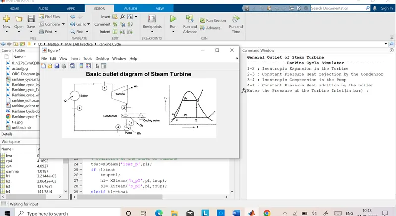
fig. Basic Outlet diagram of Steam Turbine
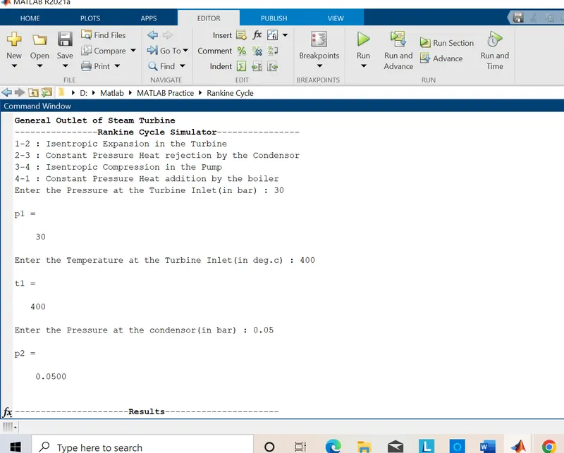
fig. Inputs by user in Command Window
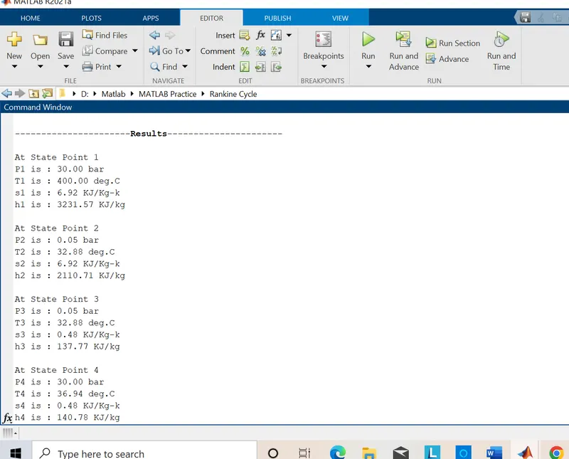
fig. State point properties
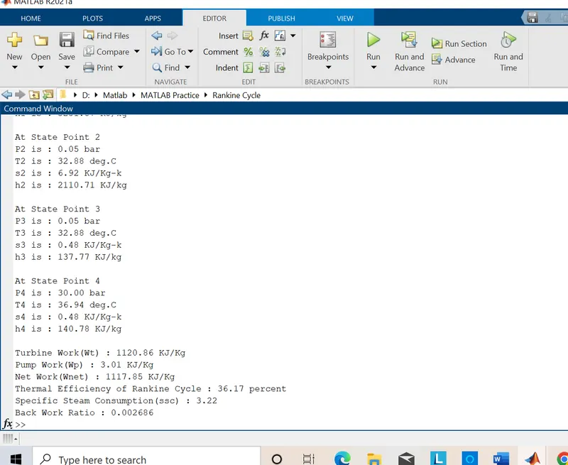
fig. Outputs of Rankine Cycle
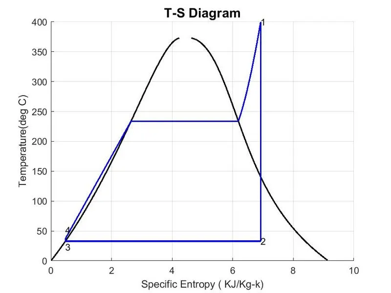
fig. Temperature-Entropy Diagram
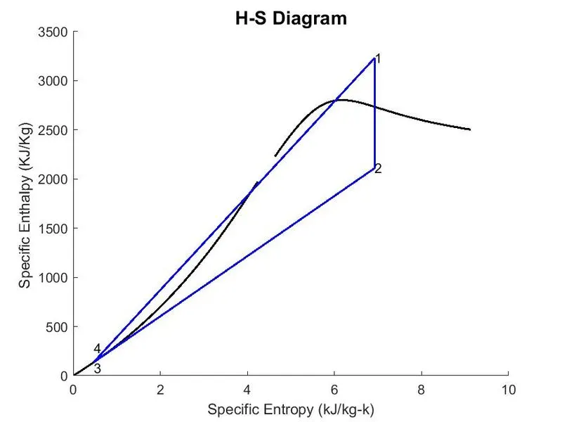
fig. Enthalpy- Entropy diagram
Conclusion :
The efficiency of the Rankine cycle can be improved in the following way:
- Reduce the average temperature
- Superheat the steam
- Increase boiler pressure
- Decrease the condenser pressure
References :